How to Develop a Credit Scoring Model with Machine Learning

Data science and the use of predictive models have impacted many industries. One such industry is finance. Credit Bureaus, banks, and other institutions involved in money lending have developed credit scoring models.

Credit scoring models evaluate an individual profile by analyzing factors like their payment history, number of accounts, credit types, and other financial information, along with demographic information to create a credit score. This credit score is then used by lending firms to determine if it’s safe to lend money to an applicant.

Let’s begin learning with the next section on types of credit scoring models used in Finance.

Download Our Latest Industry Report for FREE: Data Science Skills Survey Report 2024

Types of credit scoring models used in Finance

There are several credit scoring models examples in the real world. Some of the most prominent ones are as follows-

• FICO score

The most common example of a credit scoring model is FICO. A FICO scoring model produces credit scores by giving consumers a rating between 300 and 850, with a score above 740 considered good.

Key factors considered by the FICO model are payment history, credit utilization, credit history and usage, new credit, etc. Alternative credit scoring models emphasize different factors.

In the case of FICO 10 (debuted in 2021), for example, there is no penalty on unpaid medical bills and rental history is considered a factor different from the previous version of this model and alternative credit scoring models.  

• VantageScore

The next most prominently used model is the Vantage Score Model, which debuted in 2006 to compete with FICO. It also looks at several crucial factors like credit card balance, status of new credit obligations, number of bank accounts, etc. This model emphasizes payment history, age, and type of credit, while the customer’s recent behavior is given less weightage.

Apart from these two, several less prominent credit models exist, such as CreditXpert, Experian’s National Equivalency, and TransRisk.  

• CreditXpert

CreditXpert aims to aid businesses in evaluating prospective account holders. By scrutinizing credit histories, it seeks methods to boost scores or identify inaccuracies swiftly. Enhancing these scores can result in increased approval rates for customer loans.

• Experian’s National Equivalency Score

This model assigns users with a credit score ranging from 0 to 1,000. It considers factors such as credit length, mix, utilization, payment history, total balances, etc. However, Experian has not disclosed the specific criteria or their weights regarding calculating the score.

• TransRisk score

This model relies on information sourced from TransUnion. It is designed to evaluate a customer’s risk specifically for new accounts rather than existing ones. The TransRisk score, however, is underutilized by lenders due to its specialized focus (as limited information about the score is accessible). It has been found that in most cases, individuals’ TransRisk scores tend to be considerably lower than their FICO scores.

If you understand credit scoring models, let’s start building one. We will discuss a few guidelines for building such a model, but before that, a short note:

Credit Risk Scoring: Approach guidelines

The credit scores can hugely impact an individual’s financial and personal life. Therefore, several guidelines have been set for building a credit score model. For example, such models should be transparent and unbiased. The data used for model building should be of high quality. However, developers must consider privacy and regulatory compliance to obtain high-quality data. Overall, a credit scoring model must be unbiased and robust to anomalies.

The World Bank has written a detailed document that outlines the guidelines for credit scoring approaches, explains the importance of effective credit risk assessment in financial institutions, and discusses the various methods for evaluating creditworthiness, including traditional scoring models and newer, more sophisticated techniques.

As you can see, several ways exist of creating a credit scoring model. Let’s examine the most crucial types.

 Types of data used in Credit Scoring models

Credit scoring models can be divided into several categories. 

• Individual Scoring

Firstly, individual customer scoring models assess individuals’ creditworthiness based on several demographic factors (age, education, experience, etc.) and financial characteristics (recurring expenses, outstanding debt, etc.). Such a model can further be divided into the type of product, such as credit card or mortgage, with the latter being more comprehensive than the former.

• Enterprise Scoring

Another category of credit risk models is Enterprise Scoring, where companies are assessed. Such business credit scoring models evaluate a company’s structure, competition, employee status, source of financing, etc. For smaller companies, the owner’s profile is also examined.

• Internal and External Scoring

Credit models can also be differentiated based on the type of developers. They can be internal (developed by banks for their customers and loan applicants) or external (provided by specialized institutions like credit bureaus).

The World Bank guidelines point towards using different credit scoring model methodologies, with the primary categories being traditional and modern. In the next section, we will discuss both these types of models.

Traditional vs. Modern Credit Scoring Models

Until recently, most credit risk scoring models were based on analyzing past payment patterns using linear and logistic regression statistical algorithms. This method allowed different weights to be found for different factors. Models created using such methods are called traditional credit scoring models.

With the advent of smartphones, the availability of the internet, and several other factors, new kinds of data are now available. The data can now be semi-structured, unstructured, and huge, but it can provide a much more granular understanding of the customer and their creditworthiness. This is where new modern credit scoring models that use machine learning algorithms and deep neural networks have come into play. Such models can detect patterns and can provide a much more reliable score. The issue, however, with them is that they are much less interpretable and, therefore, can be biased.

Also read:

• Fundamentals Concepts of Neural Networks & Deep Learning
• Different Types of Machine Learning Algorithms

Given the extensive work being done in the world of credit scoring models, we will now examine how they impact business.

How do credit risk models add value to business?

In the financial business world, credit scoring models play a crucial role. It adds value to business in the following manner-

• Credit Risk Management

Credit Risk Models allow lenders to evaluate the creditworthiness of individuals and organizations and ensure that their exposure to liability is manageable. This allows lenders to assess the level of risk in their loan portfolio.

• Regulatory compliance

Today, credit risk models are required by law. Basel III (a set of international banking regulations) requires banks to use such models to meet regulatory requirements, where they are expected to maintain a certain amount of capital based on the credit risk exposure indicated by the credit risk model.

• Scenario Analysis

Stress testing can be done through credit score models, which allow lending firms to analyze various scenarios and test the resilience of their loan portfolio. This, in turn, helps manage losses in case of events like recessions and other financial crises. 

Credit risk models also allow lending firms to stay competitive, reduce costs, and mitigate risk. As you can see, several credit score models are used. However, some serious downsides must be discussed along with their various upsides.

Limitations of Credit Scoring Models

One must know the limitations when developing and deploying a credit risk model. Some of the key ones are as follows-

• Devoid of Context

Credit scoring models don’t factor in the current economic conditions, as a borrower with a high score may default, given that the economic conditions change for the worse. They also don’t consider individuals’ life events, market trends, and other macroeconomic factors.

• Dependent on Data

Such models are highly dependent on the quality of data and its availability, as gaps and anomalies in the data can greatly adversely impact the model’s accuracy. There is an overreliance on historical data when building such models, and a customer’s recent change in behavior is often overlooked.

• Biased

Often, such models are biased toward certain demographic groups and credit applicants. This is often systemic discrimination in the historical data that passes to the models.

• Susceptible to Fraud

If one knows the loopholes in calculating the credit score, individuals can manipulate their creditworthiness, making such models susceptible to fraud.

• Opaque

Advanced models are often highly complex, making understanding how a score is calculated difficult. This opaqueness leads to a lack of public trust in such models and a general sense of animosity towards the financial system.

Now that all of the major aspects of credit score models have been covered, it’s time to create one of our own. 

How To Build a Credit Scoring Model [with Code]?

To build a credit scoring model, one must have the data. The data typically is historical, where information about bank customers is available, and underwriters or bank officials have already done credit scoring based on the customer’s performance.

The next steps typically include preparing the data, building and evaluating a model, and using the model to predict the credit scores of new customers or loan applicants.

Let us build a credit scoring model using one such data (you can find it at this location).

There are five core steps:

1. Importing data set
2. Exploratory data analysis
3. Data preprocessing
4. Model building
5. Implementing model on new data

The whole process has various other steps between the main steps. The workflow looks like this:

Let’s start.

01. Importing datasets

We start with importing basic libraries and historical data.

# importing pandas for reading data and performing other dataframe related operations
import pandas as pd

# importing numpy for performing various numerical operations
import numpy as np

# importing matplotlib and seaborn for visualization
import matplotlib.pyplot as plt
import seaborn as sns

# importing the historical banking data as a pandas DataFrame
historical_df = pd.read_csv('Historical_Banking_Data.csv', low_memory=False)

# creating a copy of the data for further analysis
df = historical_df.copy()

02. Exploratory Data Analysis

Understanding the data you are dealing with is crucial in credit score models. It allows you to understand what data pre-processing steps need to be taken and how the model can be built.

Read: Exploratory Data Analysis in Python

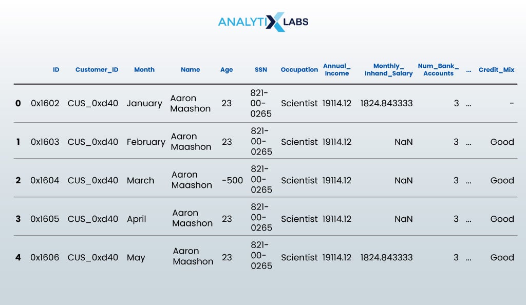
We start this by viewing the first few rows of the dataset.

df.head()

• OUTPUT:

We then find the number of rows and columns there in the data.

print("The number of rows are {} and the number of columns are {}".format(df.shape[0],df.shape[1]))

• OUTPUT:

The number of rows are 100000 and number of columns are 28

For credit score model building, we need all data to be complete and have no missing values. 

Let’s check the same:

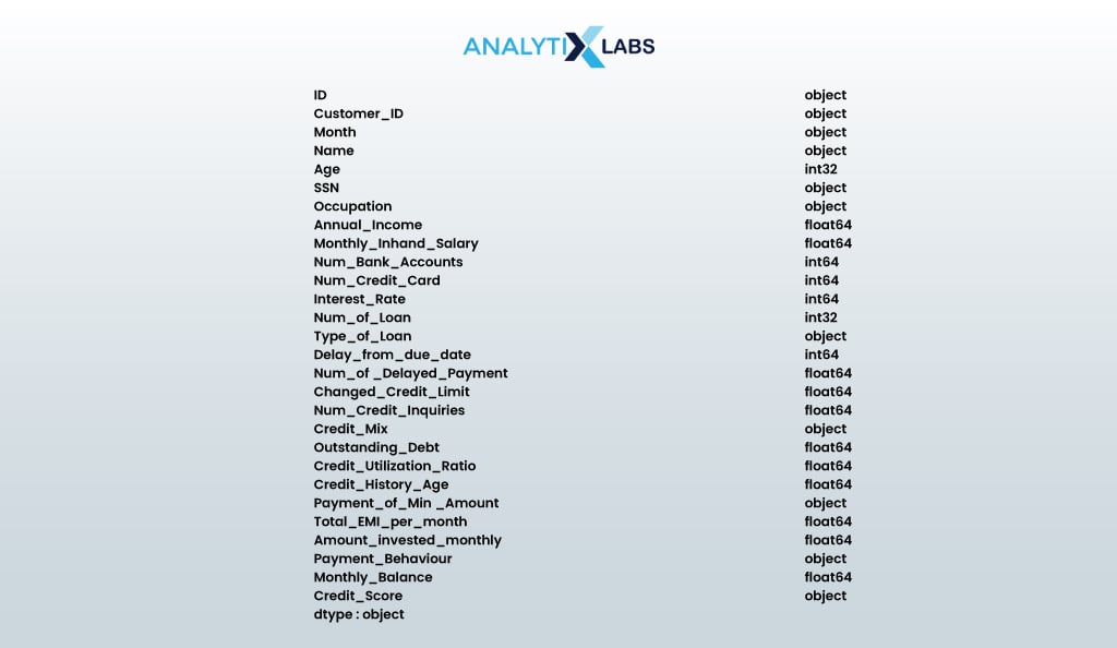
# finding the data types and number of non-null values in the data
df.info()

• OUTPUT:

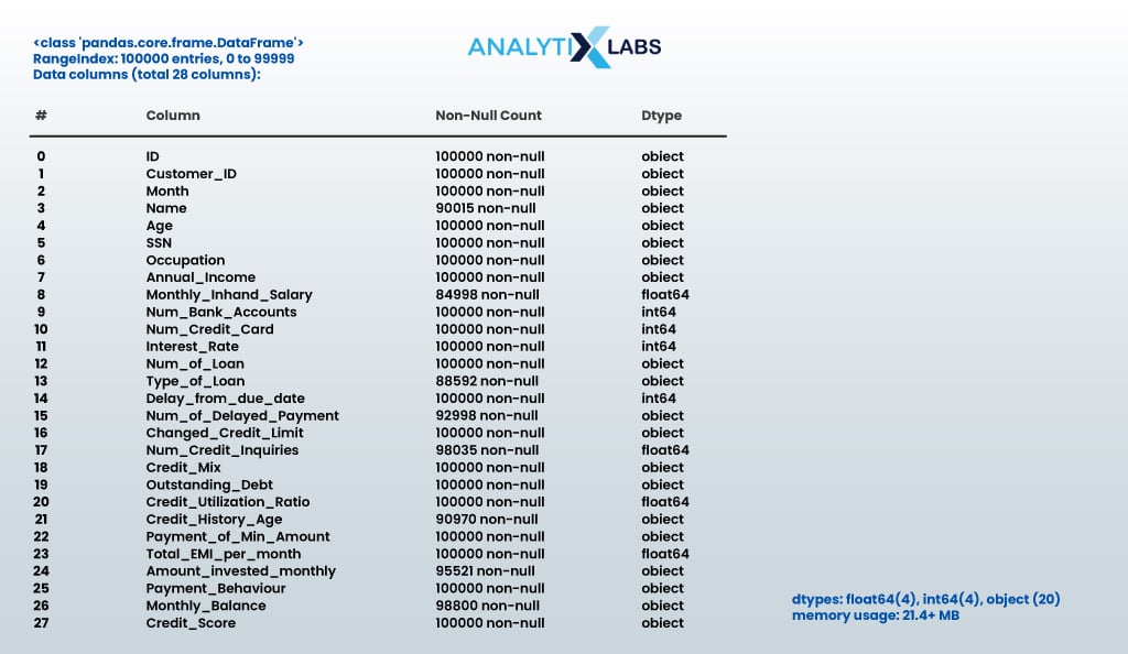
 It seems missing values are present in the dataset, and both the numerical and string-based features are present. 

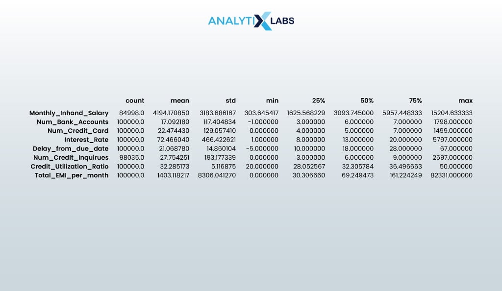
To further understand the data, let us do a basic descriptive statistical analysis of both features.

Also read: Sampling Techniques in Statistics

# finding the key statistical values of the numerical columns
df.describe().T

• OUTPUT:

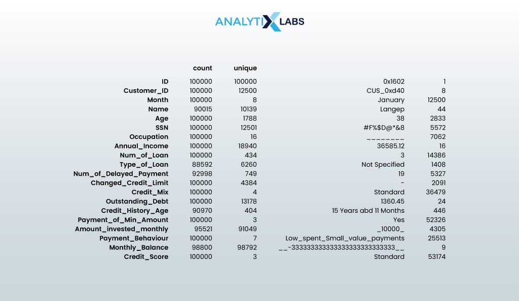
# finding the key statistical values of the categorical columns
df.describe(exclude=np.number).T

• OUTPUT:

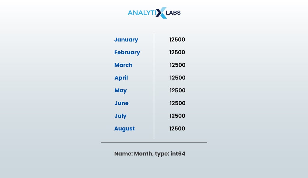
Let us also look at the contents of the month column.

df.Month.value_counts()

• OUTPUT:

Some of the key insights based on the exploratory analysis done so far are as follows-

• Customer_ID has 12500 unique values, indicating that there is information for 12500 customers.
• Only eight unique values are present for the month. It seems information for all the 125000 customers is retrieved every month and is done from January to August.
• Age has 1788 unique values; therefore, it looks anomalous.
• The number of SSN and Customer ID values don’t match, which means there are problems in the column.
• Data types seem incorrect due to invalid values being present in the data. E.g., Credit_History_Age or Amount_invested_monthly has data type as “object” due to non-numerical values in the columns.

As expected, the data is unclean and full of issues. We first focus on removing the missing values and correcting the data type. To do so, we need to find all the unwanted values in the different columns that cause them to have incorrect data types.

# finding the unique values for each column in the data to find unwanted values
# first creating a copy of the data that do not have missing values
df_without_na = df.dropna().copy()

# finding the unique values for each column
for i in df_without_na:
print('\n', i, df_without_na[i].unique())

• OUTPUT:

This is the most onerous aspect of building a credit-scoring model. We must now carefully analyze each column to determine what is wrong with it and what correcting measures must be taken.

​

#	Columns Name	Current Data Type	Required Type	Description	Unwanted Value	Findings
1	ID	object	object (ID)	ID of every observation	None	No missing values. It may not be useful for modeling.

03. Data Preprocessing

The next step in a credit model-building project is to perform data preprocessing to make the data suitable for model-building. In this step, we will impute missing values, correct data types, cap outliers, visualize key features, reduce the dataset’s dimensionality and multicollinearity, and encode, normalize, and split data into train and test.

03.1. Missing value imputation and typecasting

Based on the analysis, it was found that several columns have missing values and unwanted values that are sometimes concatenated with the correct values, making it difficult to perform missing value imputation.

Below, I have created a user-defined function that removes unwanted values and performs grouped Missing Value Imputation (MVI).

The idea behind a grouped missing value imputation is to perform missing value imputation using a mode where the data can be grouped by customer ID, and the information of the same customer can (from other months’ data) be used to impute a missing value regarding the customer.

ef preprocess_data(data, mvi_groupby=None, mvi_customval=None, column=None, unwanted_value_replace=None, unwanted_value_strip=None, datatype=None):

# stripping unwanted values that might be at the beginning or end of the value
if unwanted_value_strip is not None:
if data[column].dtype == object:
data[column] = data[column].str.strip(unwanted_value_strip)
print(f"\nTrailing & leading {unwanted_value_strip} are removed")

# replacing unwanted value with NaN
if unwanted_value_replace is not None:
data[column] = data[column].replace(unwanted_value_replace, np.nan)
print(f"\nUnwanted value {unwanted_value_replace} is replaced with NaN")

# performing missing value imputation (mvi) using mode after grouping data using the column specified by the user
if mvi_groupby and column:
data[column] = data[column].replace('', np.nan)
group_mode = data.groupby(mvi_groupby)[column].transform(lambda x: x.mode().iat[0])
data[column] = data[column].fillna(group_mode)
print("\nMissing values imputed with group mode")

# performing missing value imputation using a user provided custom value
if mvi_customval is not None:
data[column] = data[column].replace('', np.nan)
data[column].replace([np.NaN], mvi_customval, inplace=True)
print(f"\nMissing values are replaced with '{mvi_customval}'")

# changing the data type of the column based on user provided data type
if datatype is not None:
data[column] = data[column].astype(datatype)
print(f"\nDatatype of {column} is changed to {datatype}")

print('----------------------------------------------------')

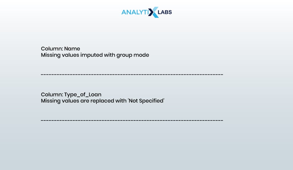
We start by performing MVI on the categorical columns.

print("Column: Name")
preprocess_data(data = df,
column = 'Name',
mvi_groupby = 'Customer_ID')

print("Column: Type_of_Loan")
preprocess_data(data = df,
column = 'Type_of_Loan',
mvi_customval = 'Not Specified')

• OUTPUT:

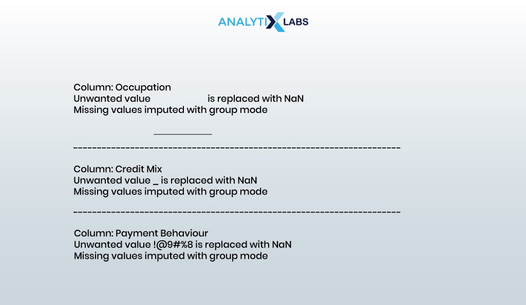
Let us also replace unwanted values and perform MVI.

print("Column: SSN")
preprocess_data(data = df,
column = 'SSN',
unwanted_value_replace = '#F%$D@*&8',
mvi_groupby = 'Customer_ID')
print("Column: Occupation")
preprocess_data(data = df,
column = 'Occupation',
unwanted_value_replace = '_______',
mvi_groupby = 'Customer_ID',)

print("Column: Credit_Mix")
preprocess_data(data = df,
column = 'Credit_Mix',
unwanted_value_replace = '_',
mvi_groupby = 'Customer_ID')

print("Column: Payment_Behaviour")
preprocess_data(data = df,
column = 'Payment_Behaviour',
unwanted_value_replace = '!@9#%8',
mvi_groupby = 'Customer_ID')

• OUTPUT:

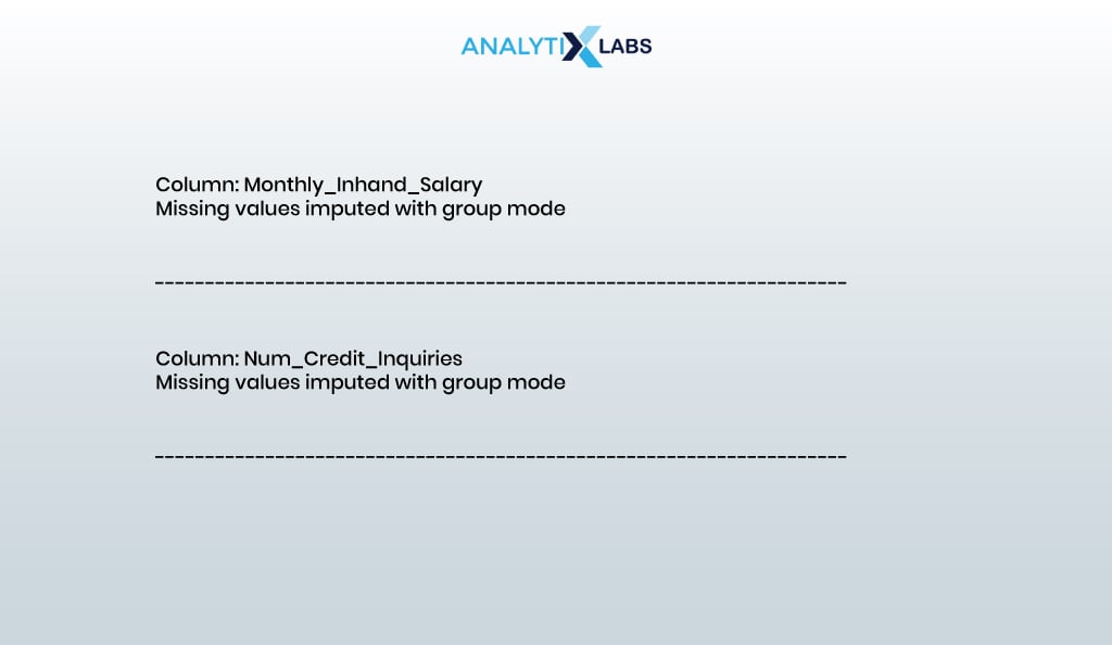
We will now perform MVI on numerical columns.

print("Column: Monthly_Inhand_Salary")
preprocess_data(data = df,
column = 'Monthly_Inhand_Salary',
mvi_groupby = 'Customer_ID')

print("Column: Num_Credit_Inquiries")
preprocess_data(data = df,
column = 'Num_Credit_Inquiries',
mvi_groupby = 'Customer_ID')

• OUTPUT:

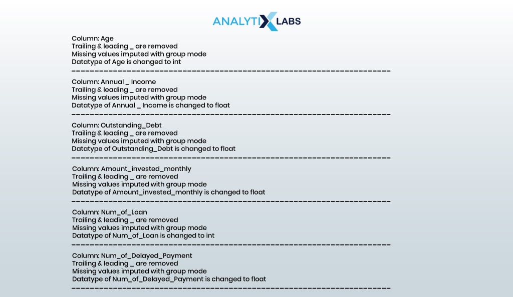
We will now strip the unwanted values and perform MVI and type casting.

print("Column: Age")
preprocess_data(data = df,
column = 'Age',
unwanted_value_strip = '_',
mvi_groupby = 'Customer_ID',
datatype = 'int')

print("Column: Annual_Income")
preprocess_data(data = df,
column = 'Annual_Income',
unwanted_value_strip = '_',
mvi_groupby = 'Customer_ID',
datatype = 'float')

print("Column: Outstanding_Debt")
preprocess_data(data = df,
column = 'Outstanding_Debt',
unwanted_value_strip = '_',
mvi_groupby = 'Customer_ID',
datatype = 'float')

print("Column: Amount_invested_monthly")
preprocess_data(data = df,
column = 'Amount_invested_monthly',
unwanted_value_strip = '_',
mvi_groupby = 'Customer_ID',
datatype = 'float')

print("Column: Num_of_Loan")
preprocess_data(data = df,
column = 'Num_of_Loan',
unwanted_value_strip = '_',
mvi_groupby = 'Customer_ID',
datatype = 'int')

print("Column: Num_of_Delayed_Payment")
preprocess_data(data = df,
column = 'Num_of_Delayed_Payment',
unwanted_value_strip = '_',
mvi_groupby = 'Customer_ID',
datatype = 'float')

• OUTPUT:

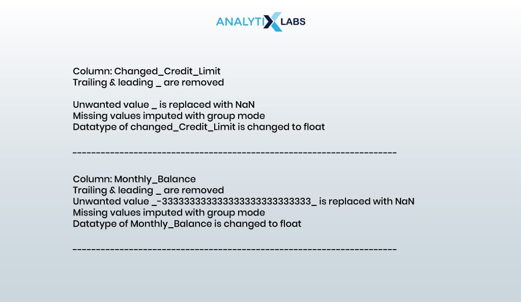
Next, we not only strip unwanted values attached to the actual values (e.g., “_7272”) but also replace the unwanted values (e.g., “__-333333333333333333333333333-”) with NaN and perform MVI and type casting.

print("Column: Changed_Credit_Limit")
preprocess_data(data = df,
column = 'Changed_Credit_Limit',
unwanted_value_strip = '_',
unwanted_value_replace = '_',
mvi_groupby = 'Customer_ID',
datatype = 'float')
print("Column: Monthly_Balance")
preprocess_data(data = df,
column = 'Monthly_Balance',
unwanted_value_strip = '_',
unwanted_value_replace = '__-333333333333333333333333333__',
mvi_groupby = 'Customer_ID',
datatype = 'float')

• OUTPUT:

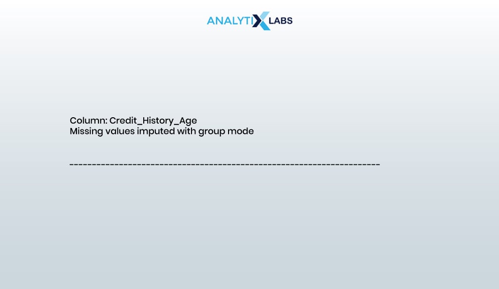
Lastly, we correct the ‘Credit_History_Age’ column where age is presented as “22 Years and 4 Months” and change it to show the information in the number of months.

# creating a function that picks the year and month and then combines them to give total number of months
def credit_history_in_months(val):
if pd.notnull(val):
years = int(val.split(' ')[0])
month = int(val.split(' ')[3])
return (years*12)+month
else:
return val

# applying the function to the column
df['Credit_History_Age'] = df['Credit_History_Age'].apply(lambda x: credit_history_in_months(x)).astype(float)

print('Column: Credit_History_Age')
preprocess_data(data = df,
column = 'Credit_History_Age',
mvi_groupby = 'Customer_ID')

• OUTPUT:

Time to now check if there are missing values left.

df.isna().sum()

• OUTPUT:

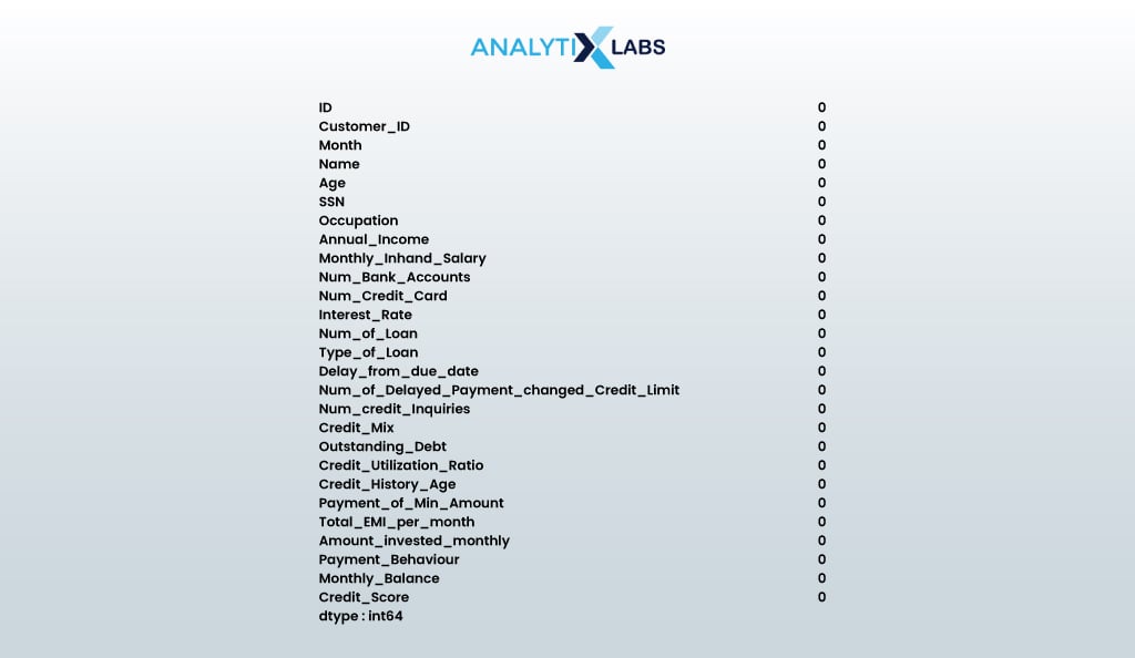
It seems that there are no missing values left. Let’s final-check the data types to see if they are as expected.

df.dtypes

• OUTPUT:

03.2. Outlier capping

The next step in data preprocessing is to find and cap outliers. Let us create a function that finds and caps outliers using the Inter-Quartile (IQR) method. 

ef outlier_capping(data, threshold=1.5):

# making a copy of the input DataFrame
data_copy = data.copy()

# creating a empty list to save the outlier indices
outlier_indices = []

# calculating quartile 1 and 3 for every numerical column in the data
for column in data_copy.columns:
if pd.api.types.is_numeric_dtype(data_copy[column]):

# calculating quartiles
Q1 = data_copy[column].quantile(0.25)
Q3 = data_copy[column].quantile(0.75)

# calculating inter-quartile range
IQR = Q3 - Q1

# defining the upper and lower outlier bounds
lower_bound = Q1 - threshold * IQR
upper_bound = Q3 + threshold * IQR

# identifying outliers
outliers = data_copy[(data_copy[column] < lower_bound) | (data_copy[column] > upper_bound)] outlier_indices.extend(outliers.index)

# capping outliers
data_copy[column] = np.where(data_copy[column] < lower_bound, lower_bound, data_copy[column]) data_copy[column] = np.where(data_copy[column] > upper_bound, upper_bound, data_copy[column])

# removing duplicates from outlier_indices list
outlier_indices = list(set(outlier_indices))

# returning the dataframe with capped outliers
return data_copy, outlier_indices

# running the function to cap all the outliers in the data
df_clean, outliers = outlier_capping(df)

To check if outlier capping has worked, we will create boxplots for every column before and after outliers were capped to perform a comparative study.

# comparing the columns with and without the outliers
def outlier_capping_comparison(data, data_processed, outlier_indices):
for column in data.columns:
if pd.api.types.is_numeric_dtype(data[column]):
plt.figure(figsize=(12, 6))

# plotting the numerical columns from the original dataframe
plt.subplot(1, 2, 1)
sns.boxplot(data=data[column])
plt.title(f'Before Outlier Capping : {column}')

# plot distribution of the numerical columns where outliers are capped
plt.subplot(1, 2, 2)
sns.boxplot(data=data_processed[column])
plt.title(f'After Outlier Capping : {column}')

# showing output
plt.tight_layout()
plt.show()

# running the function to compare the numerical columns before and after outlier capping
outlier_capping_comparison(data = df, data_processed = df_clean, outlier_indices = outliers)

• OUTPUT:

It’s evident that outlier capping was useful and effective, as several outliers previously had data that are now gone.

03.3. Visualization

As the data is free of missing values and outliers and has proper data types, we can perform some advanced EDA by visualizing it.

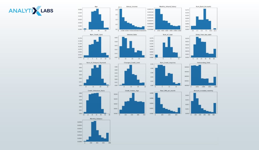
We create a histogram for the numerical columns to understand their distribution.

df_clean.hist(figsize=(20, 20), grid=False, density=True)
plt.show()

• OUTPUT:

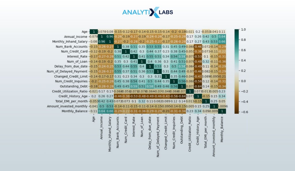
Next, we create a correlation matrix to have a brief idea of the level of multicollinearity in the data.

plt.figure(figsize=(10,5))
corr_matrix = df_clean.corr()
sns.heatmap(corr_matrix, cmap="BrBG", annot=True)
plt.show()

• OUTPUT:

It’s time to check if we are dealing with balanced data, which we do by understanding the distribution of the target variable using a pie chart.

credit_socre_vals = df_clean.Credit_Score.value_counts().index
credit_socre_labels = df_clean.Credit_Score.value_counts().values

plt.pie(data = df_clean,
x = credit_socre_labels,
labels = credit_socre_vals,
autopct = '%1.1f%%',
shadow = True,
radius = 1)

plt.show()

• OUTPUT:

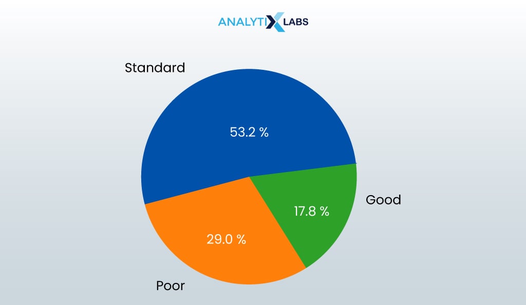
The data seems unbalanced. Next, we create a few bar charts to understand the interactions between categorical columns.

def create_stacked_bar_crosstab(data, cat_col1, cat_col2, rotation_val=0):

# creating cross tab between two variables
pd.crosstab(data[cat_col1], data[cat_col2]).plot(kind='bar', stacked=True)

# adding title
plt.title(f'{cat_col1} & {cat_col2} Distribution')

# adding x and y label
plt.xlabel(f'{cat_col1}')
plt.ylabel('Number of Observations')

# option for rotating xticks
plt.xticks(rotation = rotation_val)

plt.show()

Next, we will understand the interaction between occupation and credit score.

create_stacked_bar_crosstab(data = df_clean,
cat_col1 = 'Occupation',
cat_col2 = 'Credit_Score',
rotation_val = 90)

• OUTPUT:

We will also explore the interaction between payment behavior and credit score.

create_stacked_bar_crosstab(data = df_clean,
cat_col1 = 'Payment_Behaviour',
cat_col2 = 'Credit_Score',
rotation_val=78)

• OUTPUT:

As the data is relatively clean, much visualization is possible at this stage. For example, scatterplots and bar plots can be created to understand the interaction between numerical-numerical and numerical-categorical columns. 

03.4. Encoding

To create a credit score model, the data must be represented numerically. Therefore, encoding must be performed because the data has mixed data types. I perform label encoding for ordinal and one-hot encoding for nominal categorical columns. 

Let us start by converting the Month column by replacing the month name with the month number.

df_clean['Month'] = pd.to_datetime(df_clean.Month, format='%B').dt.month

We now find the number of unique values in the different categorical columns.

categorical_cols = ['Occupation', 'Type_of_Loan', 'Credit_Mix', 'Payment_of_Min_Amount', 'Payment_Behaviour'] for column in categorical_cols:
unique_values_count = len(df_clean[column].unique())
print(f"Number of unique values in the '{column}' column:", unique_values_count)

• OUTPUT:

Now, we perform label encoding ‘Type_of_Loan’ as creating dummy variables will cause dimensionality issues.

from sklearn.preprocessing import LabelEncoder
label_encoder = LabelEncoder()
df_clean['Type_of_Loan'] = label_encoder.fit_transform(df_clean['Type_of_Loan'])

Now encode the column ‘Payment_of_Min_Amount’.

# finding the unique values
print('Unique values in Payment_of_Min_Amount are: ', df_clean['Payment_of_Min_Amount'].unique())

• OUTPUT:

We perform label encoding ‘Payment_of_Min_Amount’ as it seems ordinal.

# setting values
target_mapping = {'No': 1, 'NM': 2, 'Yes': 3}

# mapping values
df_clean['Payment_of_Min_Amount'] = df_clean['Payment_of_Min_Amount'].map(target_mapping)

We will now perform one hot encoding on the remaining categorical columns as they all seem of nominal type.

# mentioning the categorical columns where one-hot encoding needs to be performed
columns_to_encode = ['Occupation', 'Credit_Mix', 'Payment_Behaviour']

# creating dummy variables
df_dummy = pd.get_dummies(df_clean[columns_to_encode])

# concatenating the dummy variables with the original dataframe
df_processed = pd.concat([df_clean, df_dummy], axis=1)

# dropping the original categorical columns for which dummy variables were created
df_processed.drop(columns_to_encode, axis=1, inplace=True)

Finally, we now encode the target variable.

target_mapping = {'Poor': 1, 'Standard': 2, 'Good': 3}
df_processed['Credit_Score'] = df_processed['Credit_Score'].map(target_mapping)

It’s time to check if any string-based column is left in the data.

df_processed.dtypes[df_processed.dtypes=='object']

• OUTPUT:

Finally, all the features in the data are now numerical.

03.5. Feature reduction

Currently, the data contains several independent features, and they may all be useless for modeling as they may have a weak relationship with the target variable. Therefore, we will remove unwanted features and select the important ones.
We start by dropping columns irrelevant to building a credit-scoring model.

df_clean.drop(['ID', 'Customer_ID', 'SSN', 'Name'], axis=1, inplace=True)

We now find the important variables using tree-based and statistical methods like Random Forest, Recursive Feature Elimination (RFE), and Univariate Analysis.

# importing key libraries
from sklearn.ensemble import RandomForestClassifier
from sklearn.feature_selection import RFE, SelectKBest, f_classif

# extracting the predictor variables
X = df_processed.drop('Credit_Score', axis=1)

# extracting the target variable
y = df_processed['Credit_Score']

# Method 1: finding feature importance using Tree-Based method
rf_model = RandomForestClassifier()
rf_model.fit(X, y)
feature_importances = rf_model.feature_importances_
top_10_rf = X.columns[feature_importances.argsort()[-10:][::-1]]

# Method 2: using Recursive Feature Elimination (RFE)
rfe_selector = RFE(estimator=RandomForestClassifier(), n_features_to_select=10, step=1)
rfe_selector.fit(X, y)
top_10_rfe = X.columns[rfe_selector.support_]

# Method 3: using Univariate Feature Selection
selector = SelectKBest(score_func=f_classif, k=10)
selector.fit(X, y)
top_10_univariate = X.columns[selector.get_support()]

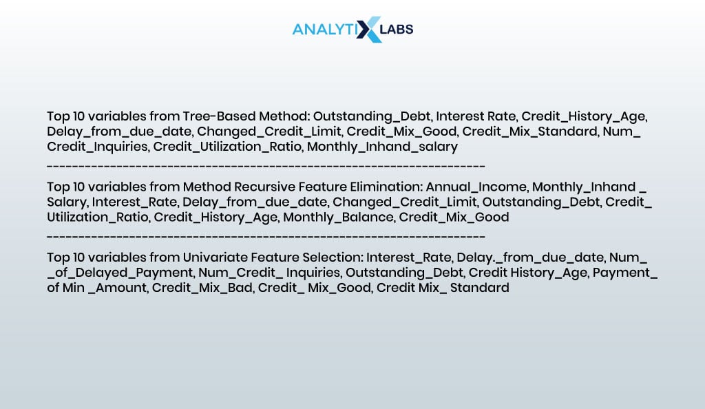
The following are the top 10 variables from each method.

print("Top 10 variables from Tree-Based Method:", ', '.join(top_10_rf))
print("---------------------------------------------------------------------------------------------------------")
print("Top 10 variables from Method Recursive Feature Elimination:", ', '.join(top_10_rfe))
print("---------------------------------------------------------------------------------------------------------")
print("Top 10 variables from Univariate Feature Selection:", ', '.join(top_10_univariate))

• OUTPUT:

We find the important columns by picking only those that appear in at least one of the feature selection method’s outputs.

imp_columns = list(set(top_10_rf.tolist() + top_10_rfe.tolist() + top_10_univariate.tolist()))
imp_columns

• OUTPUT:

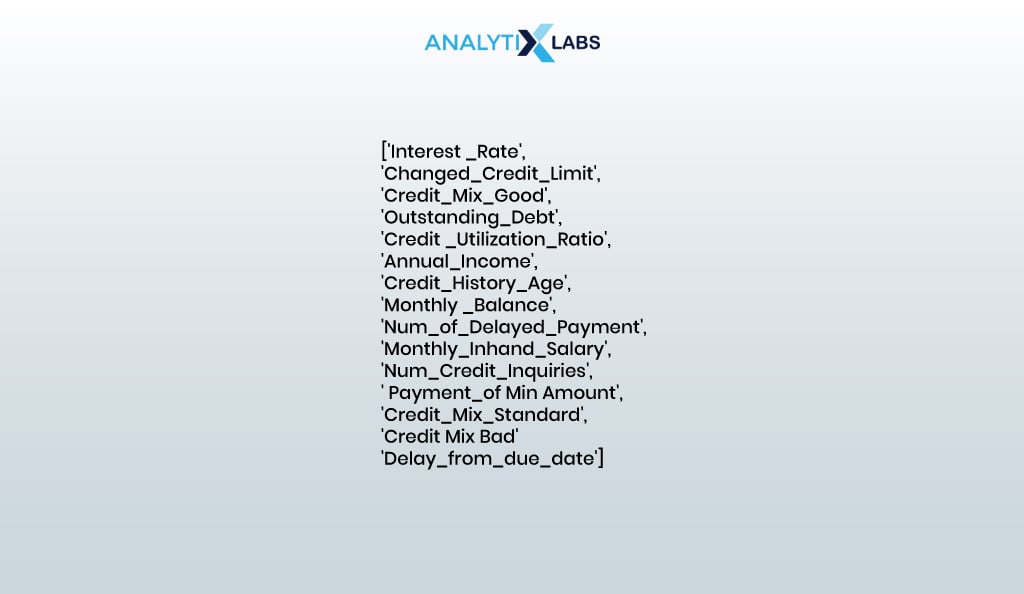
So far, 15 columns have been identified to be important.

print('Number of selected columns are: ', len(imp_columns))

• OUTPUT:

No. of selected columns are: 15

03.6. Checking multicollinearity

Some of the current 15 features might be related, causing multicollinearity. We, therefore, find and drop such features.

• Correlation matrix: We use correlation to check for multicollinearity and mark the columns where the absolute correlation value is above 0.7.

# extracting the selected independent features
X_selected = df_processed[imp_columns]

# creating correlation matrix
correlation_matrix = X_selected.corr()

# finding highly correlated feature pairs
highly_correlated_pairs = (correlation_matrix.abs() > 0.7) & (correlation_matrix.abs() < 1)

print("Highly correlated pairs of variables and their correlation values:\n")
checked_pairs = set() # To keep track of checked pairs
for col1 in X_selected.columns:
for col2 in X_selected.columns:
if col1 != col2 and (col1, col2) not in checked_pairs and (col2, col1) not in checked_pairs:
if highly_correlated_pairs.loc[col1, col2]:
correlation_value = correlation_matrix.loc[col1, col2] print(f"{col1} - {col2}: {correlation_value:.2f}")
checked_pairs.add((col1, col2))

• OUTPUT:

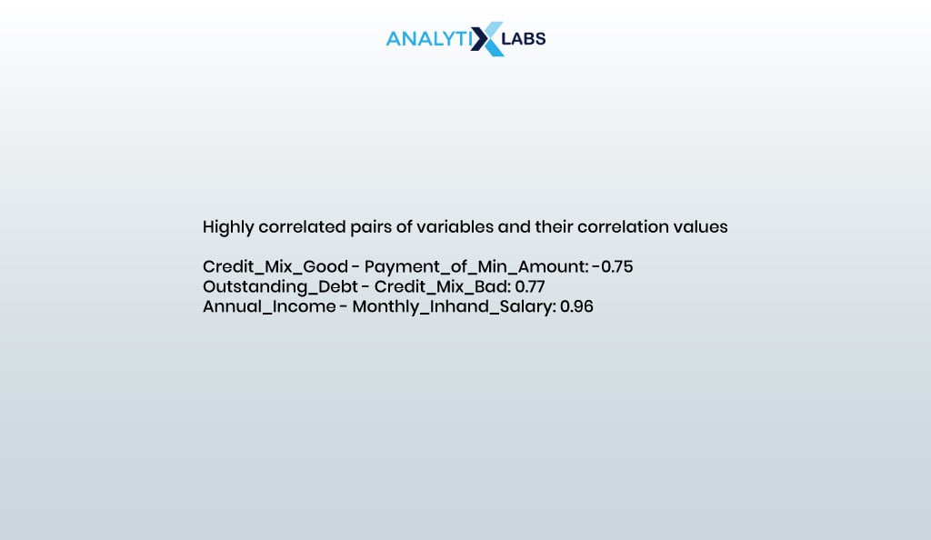
We now remove the correlated columns.

X_selected.drop(['Annual_Income', 'Credit_Mix_Good', 'Credit_Mix_Bad'], axis=1, inplace=True)

• Variance inflation factor (VIF): To eliminate multicollinearity, we will calculate the VIF value for each independent feature.

# importing library for calculating vif
from statsmodels.stats.outliers_influence import variance_inflation_factor

# calculating vif ofthe selected features
vif_df = pd.DataFrame()
vif_df["Variable"] = X_selected.columns
vif_df["VIF"] = [variance_inflation_factor(X_selected.values, i) for i in range(X_selected.shape[1])] print("Variance Inflation Factors:")
print(vif_df)

• OUTPUT:

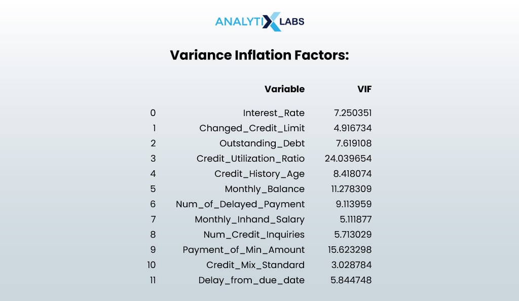
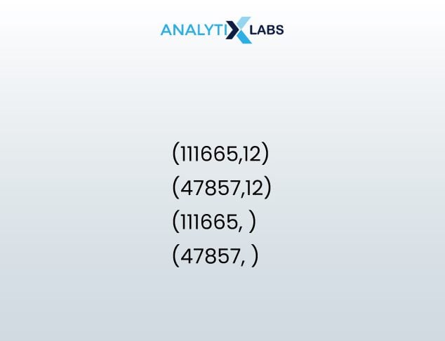
It seems that multicollinearity is under control, and I don’t drop variables anymore (while there are a few columns where the VIF value is above the permissible limit of 10, they are very few in numbers). Thus, the final number of important independent columns is 12.

print('Number of selected columns are: ', len(X_selected.columns))

• OUTPUT:

No. of selected columns are: 12

This makes the final list of predictors to be-

final_X_cols = X_selected.columns.tolist()
print("Final selected predictors are: ", ', '.join(final_X_cols))

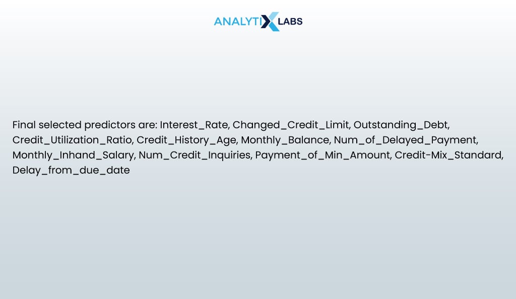
We now create the final dataset for modeling with the twelve selected independent features and the target (dependent) variable.

df_final = df_processed[final_X_cols + ['Credit_Score']]

03.7. Scaling data

The independent features need to be normalized to use the data for modeling. I do this using the min-max scalar method.

# splitting the predictors and target
X = df_final.drop('Credit_Score',axis=1)
y = df_final['Credit_Score']

# normalizing data using min-max scaler
from sklearn.preprocessing import MinMaxScaler

# initializing min-max scaler
scaler = MinMaxScaler()

# fitting it onto the independent features
X = scaler.fit_transform(X)

03.8. Balancing data

We are dealing with class-imbalanced data, as evidenced by the number of categories in the target feature.

y.value_counts()

• OUTPUT:

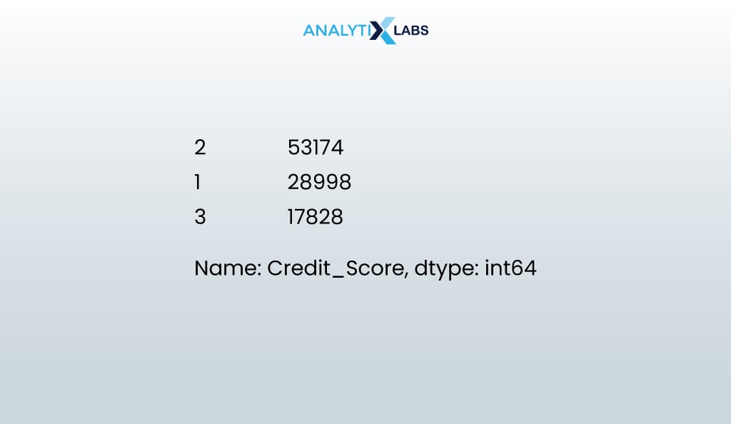
Note that currently, the number of rows (observations) is 100,000.

len(X)

• OUTPUT: 100000

We used the SMOTE method, where synthetic samples are created for the minority classes to balance the classes.

# importing SMOTE library
from imblearn.over_sampling import SMOTE

# initializing SMOTE
smote = SMOTE()

# fitting SMOTE to the data
X_bal, y_bal = smote.fit_resample(X, y)

The new count of the different categories in the target feature is the same.

y_bal.value_counts()

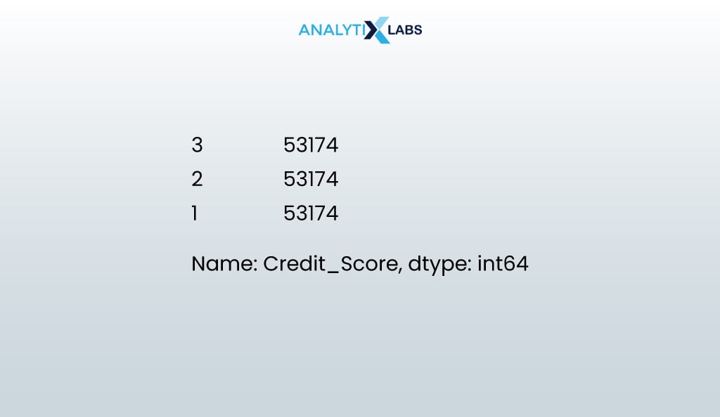
Notice how the number of observations has increased from the previous count of 100,000 due to synthetic rows being created.

len(X_bal)

• OUTPUT: 159522

03.9. Train-test split

Dimensionality Reduction and multicollinearity checks have been done to prevent overfitting. However, the data must be split into training and testing to ensure the credit scoring model generalizes well. This ensures that the model is trained and evaluated on separate datasets. Doing so minimizes data leakages and produces the accuracy you will see in the real world.

# importing required library
from sklearn.model_selection import train_test_split

# splitting data into train and test
X_train, X_test, y_train, y_test = train_test_split(X_bal, y_bal, test_size = 0.3, random_state=123, stratify = y_bal)

# finding number of rows and column of the train and test dataset
print(X_train.shape)
print(X_test.shape)
print(y_train.shape)
print(y_test.shape)

• OUTPUT:

04. Model Building

As the data preprocessing is done, it’s fit for model building. Thus, it is time to build a credit scoring model.

04.1. Finding best model

To build a modern credit scoring model, we can try various machine learning algorithms and perform 5-fold cross-validation to get accurate results.

# importing libraries to create different types of machine learning models
from sklearn.tree import DecisionTreeClassifier
from sklearn.ensemble import RandomForestClassifier
from sklearn.naive_bayes import GaussianNB
from sklearn.linear_model import LogisticRegression
from sklearn.neighbors import KNeighborsClassifier

# importing model evaluation libraries
from sklearn.model_selection import cross_val_score
from sklearn.metrics import accuracy_score, precision_score, recall_score, classification_report, confusion_matrix

# List of classifiers to test
classifiers = [
('Decision Tree', DecisionTreeClassifier()),
('Random Forest', RandomForestClassifier()),
('KNN', KNeighborsClassifier(n_neighbors=5)),
('Gaussion NB',GaussianNB())
]

# Iterate over each classifier and evaluate performance
for clf_name, clf in classifiers:
# Perform cross-validation
scores = cross_val_score(clf, X_train, y_train, cv=5, scoring='accuracy')

# Calculate average performance metrics
avg_accuracy = scores.mean()
avg_precision = cross_val_score(clf, X_train, y_train, cv=5, scoring='precision_macro').mean()
avg_recall = cross_val_score(clf, X_train, y_train, cv=5, scoring='recall_macro').mean()

# Print the performance metrics
print(f'Classifier: {clf_name}')
print(f'Average Accuracy: {avg_accuracy:.4f}')
print(f'Average Precision: {avg_precision:.4f}')
print(f'Average Recall: {avg_recall:.4f}')
print('-----------------------')

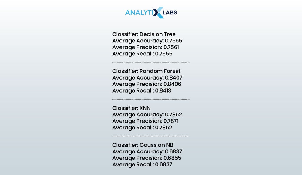
It seems that random forest has the highest accuracy value.

04.2. Fitting best model

We’ve built the random forest model by fitting it onto the training data. At this stage, several different hyperparameters can be tried out. However, we have built a relatively simple random forest model.

# initializing and fitting the random forest classifier
rf_classifier = RandomForestClassifier(n_estimators=100, random_state=42).fit(X_train, y_train)

04.3. Evaluating model

Let us now use the model on the test data and evaluate it using a confusion matrix and other performance metrics.

# making predictions on the test dataset
y_test_pred = rf_classifier.predict(X_test)

# evaluating model through a confusion matrix
cm = confusion_matrix(y_test, y_test_pred)
sns.heatmap(cm, annot=True, cmap='Blues',fmt='.0f')

plt.xlabel('Predicted Labels')
plt.ylabel('True Labels')
plt.title('Confusion Matrix')

plt.show()

• OUTPUT:

print("Classification Report")
print(classification_report(y_test, y_test_pred))

• OUTPUT:

The random forest model yielded decent results, so the credit scoring model is now complete.

05. Implementing Model on New Data

We now use our credit risk scoring model on a new dataset where the credit scores are absent.

# importing data where credit scoring needs to be done for new loan applicants
serving_df = pd.read_csv('Serving_Data_clean.csv')

# creating a copy of the serving data
df_new = serving_df.copy()

# columns in the new dataset
df_new.columns

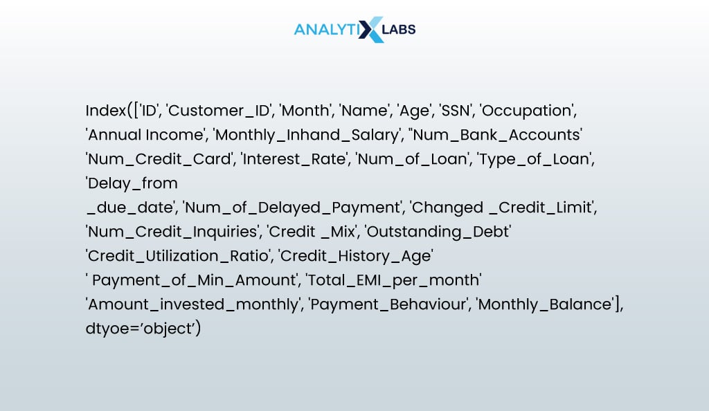
We first extract the independent features required for running the model from the data.

df_new = df_new[final_X_cols]

Given the article’s scope, we will skip the data preprocessing steps, but they will be similar to what has been done earlier. With the new data, you must remove unnecessary values, impute missing values, cap outliers, and perform typecasting, encoding, and scaling.

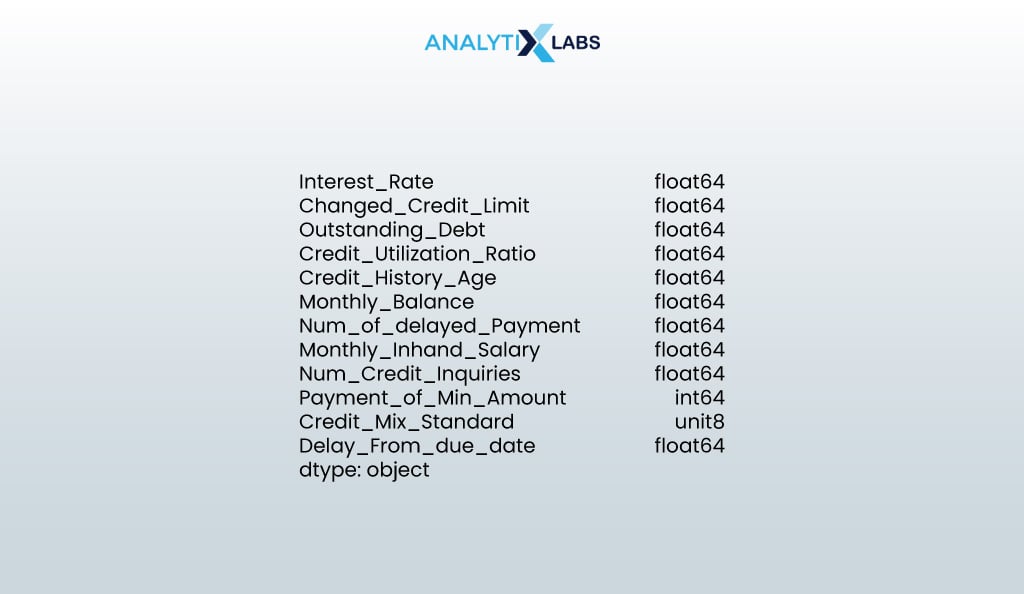
# checking if the data types are correct or not
df_new.dtypes

• OUTPUT:

# checking if there are any missing values
df_new.isna().sum()

• OUTPUT:

Let us now use the model to predict the credit scores and add them to the dataset.

# making predictions using the model
predictions = rf_classifier.predict(df_new)

# appending the predictions to the original dataset
serving_df['Credit_Score'] = pd.Series(predictions)

# viewing the final dataset with predictions
serving_df

• OUTPUT:

Thus, we have a credit risk scoring model that can predict a customer’s credit score, given specific information about the customer.

Conclusion

Developing a credit scoring model in data science is complex, with data acquisition and cleaning challenges. Yet, it’s achievable with a systematic approach and the right algorithm.

A robust model can be built by gathering and preprocessing diverse data sources, including traditional and alternative sources, and selecting an appropriate algorithm through iterative experimentation.

Continuous monitoring ensures its relevance over time, ultimately facilitating informed credit assessment.