Descriptive vs. Inferential Statistics: Definitions and Examples

Data, as we receive or see in any form, is raw, meaning the facts and figures present may or may not have structure. One field of Mathematics that can help us to mold this raw data into a structure is Statistics. The data can be summarized, analyzed, presented, and interpreted. Statistics is the art and science of collecting, organizing, analyzing, presenting and interpreting data. The branch of Statistics is further divided into sub-branches: Theoretical and Applied Statistics, and applied Statistics branches out into: Descriptive and Inferential Statistics.

In this article, we shall understand each of these branches in detail, their respective types, investigate how descriptive is different from inferential statistics, and the example of inferential and descriptive statistics.

Descriptive Statistics

Descriptive Statistics is a sub-division of Applied statistics that deals with quantifying the data. It provides a summary of the important characteristics or features of the data. It explains an event or a situation by organizing, analyzing, and presenting the data in a factual and useful way. 

Descriptive statistics talk about the data in its present form i.e. it concludes about the data that is known. The summarized data is represented using numerical and visual tools such as tables, charts, and graphs.

Let’s take a simple example of descriptive statistics for a better understanding. 

Let’s say we measure the weights of 10 students in a class. The weights are 50, 46, 56, 58.4, 62, 55, 53, 51, 48, 49. We want to find the average weight and to compute the average we shall take the sum of these 10 values and divide this sum by the total of observations in the following manner:

Average weight = [50 + 46 + 56 + 58.4 + 62 + 55 + 53 + 51 + 48 + 49]/10 = 528.4/10 = 52.84

The average weight for 10 students is 52.84.

The Methodology

The techniques used in descriptive statistics are as follows: 

• Frequency Distribution
• Measures of Central Tendency
• Measures of Variability 
• Five-Point Summary, and 
• Measure of Association between two variables

Descriptive analysis deals with describing and analysis of both single variables and bi-variables. When we want to summarize and find patterns within the same variable, then use univariate analysis to know the relationship between two variables that are referred to as bivariate analysis. 

Also read: How Univariate Analysis helps in understanding data?

For instance, the weights we saw above had weights of 10 students. Here, weight is a single variable, we found a characteristic of this variable by finding the average weight. To understand the variation in the weight variable, we can explore this further by plotting a histogram or kernel density plot (KDE). This analysis of a variable itself is known as univariate analysis and we shall dwell on this further in the upcoming Univariate analysis article. 

Let’s drill down on each of the types of descriptive statistics in the next section.

Types of Descriptive Statistics

The following methodologies that entail the types of descriptive statistics are used for summarizing the findings present within the data.

(1) Frequency Distribution

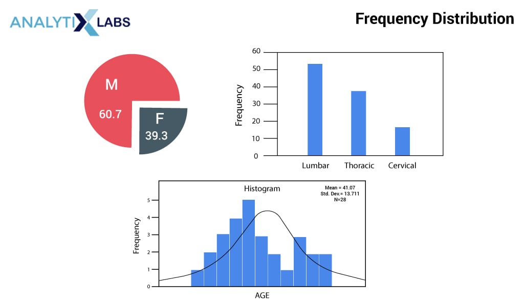
Creating a frequency distribution is the most common and simple way to visually see data in a tabular or graphical summary format. A frequency distribution can show the number or frequencies of the observations in numbers or percentages in a class interval. These class intervals must be non-overlapping, so they must be mutually exclusive and exhaustive. The relative and percent frequencies can be visually represented in a bar and pie chart.

(2) Measure of Central Tendency

Measure of central tendency refers to a single value that summarizes or describes a dataset. The USP of the measure of central tendency is that this single value represents the middle or the center value for the dataset. It indicates where most of the values within a distribution lie, which is why it is the central location of a distribution.  

It can be helpful to visualize it this way: on measuring values of similar nature, i.e., homogenous, the data tend to cluster around a mid-point or central value. It locates the distribution via various central points. This central tendency measure is a single number that represents the entire distribution or the population.

The most important measures of location or central tendency are mean, median, and mode.

• Mean

Mean is defined by the formula: Summation of all observations in a dataset divided by Total number of observations in that dataset. In mathematics, it is also called Average.

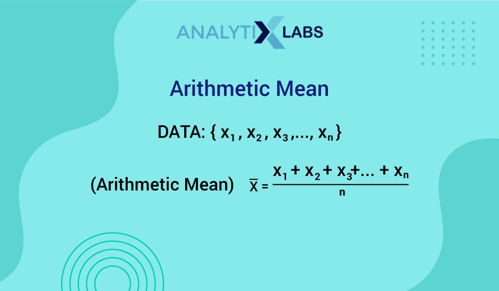
In arithmetic mean, all the observations are given the same weight implying each observation has equal importance.

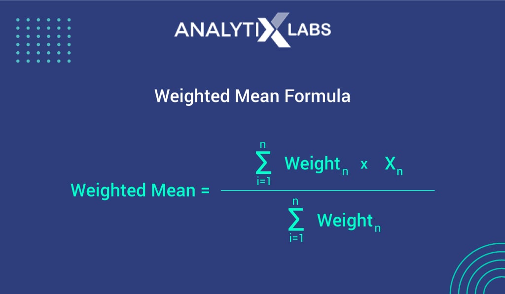
Another variation of arithmetic mean is the Weighted mean, in which each observation is given a weight that reflects its relative importance. This implies some observations may contribute that others, to account for this the weight of each observation is taken into consideration by: 

• Median

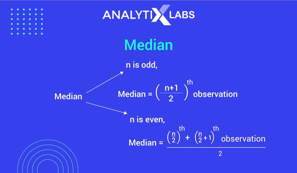
Median is the middle-value present within a data when the data is arranged in ascending order (from the smallest to largest value).

• With an odd number of observations, the median is the middle value. 
• With an even number of observations, the median is the average of the two middle values.

• Mode

The Mode occurs most often, i.e., the value with the maximum frequency of occurrence.

Median and Mode are not affected by extreme values (i.e., by outliers), whereas Mean is affected by outliers.

Though the important measures of central tendency parameters are mean, median, and Mode, other parameters also fall under Measures of location, which also help describe the data. These parameters are Percentiles and Quartiles.

Percentiles: 

A percentile gives information about how the data is spread over an interval from the smallest to the largest value. This is shown by indicating the value below which the given percentage of observations within a group fall.

The pth percentile means that at least p% of the observations are less than this value and at least (100-p) % of the observations have values greater than this value.

For example, Avinashi scored 99.78 percentile in the XAT exam. This means that the 99.78th percentile is the value (or score) below which 99.78% of the observations fall. It implies that approximately 99.78% of the students have scored less than Avinashi. In other words, 0.22% of the students have scored more than Avinashi.

Quartiles

In percentile, the division of the dataset was in two parts: pth percentile and (100-p)th percentile. Whereas in quartiles, the dataset is divided into four parts, where each part contains approximately 25% or 1/4th of the observations. These division points are referred to as Quartiles defined as:

• Q1: first quartile or 25th percentile. It comprises the lowest 25% of the observations.
• Q2: second quartile or 50th percentile. It is also known as the median, containing 0% to 50% of the observations.
• Q3: third quartile or 75th percentile. It consists of 0% to 75% of the observations.
• Q4: fourth quartile or 25th percentile. It has the highest 25% of the observations.

(3) Measures of Variability or Measure of Dispersion

Central tendency describes the central or the middle point of a dataset. Dispersion or variability describes the spread or variation present within a data. Some common ways to know how the data is dispersed are given below.

• Range

It is the simplest measure of variability. Range is computed by taking the difference between the largest (maximum) value and the smallest (minimum) value.

• Interquartile Range (IQR)

Interquartile Range(IQR) is defined as the difference between the third quartile (Q3) and the first quartile (Q1), and it is less affected by the outliers. IQR is the range for the middle 50% of the observations in the data as it is calculated after removing the highest and the lowest 25% of observations in a dataset after arranging them in ascending order.

• Variance

Variance is the averaged square deviations from each observation to the mean. It takes in all the values of the data. Variance of data is calculated by dividing the sum of the squares of each data point’s differences from the data’s average by the total number of values in the data.

A low variance implies the values in the data are closer to the mean and a higher variance indicates the data is spread out from the mean.

The difference between each observation from the mean is called the deviation of the mean.

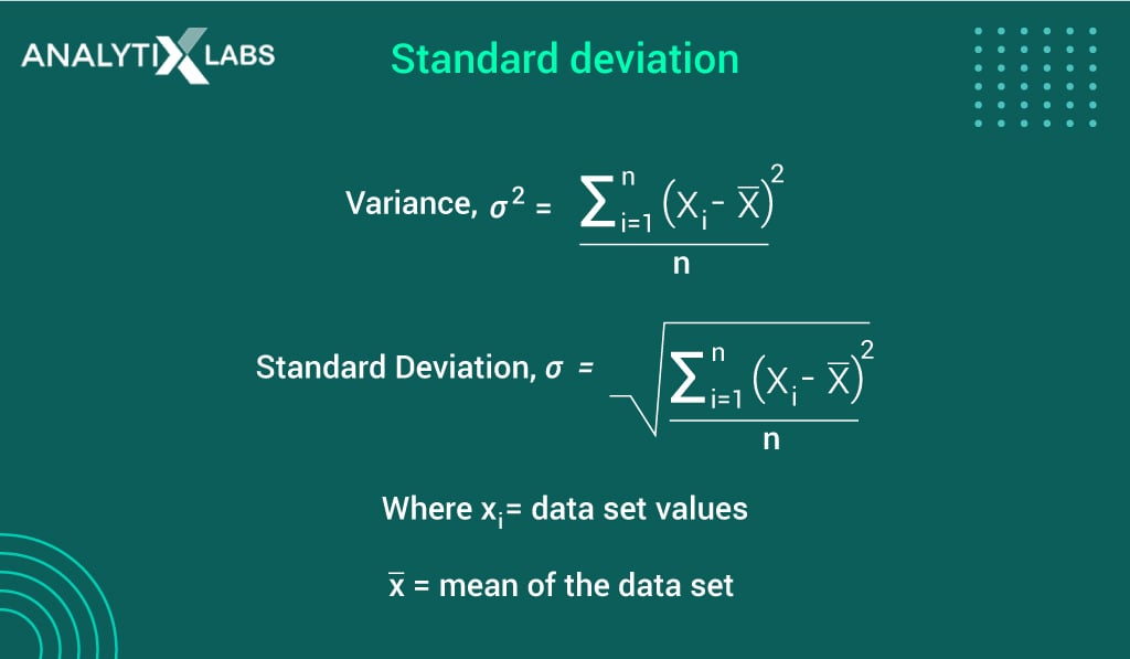
• Standard deviation

It is the positive square root of the variance. Standard deviation is denoted by sigma (σ). It implies:

• A higher standard deviation is inferred as the observations in the dataset are spread and are distant from the mean of the data.
• A lower standard deviation implies that the values are not spread and are close to the average of the dataset.

Standard deviation is fairly easier to interpret than variance because standard deviation is measured in the same units as the original values. On the other hand, variance is expressed in much larger units.

• Coefficient of Variation

The coefficient of variation is a relative measure of variability. It measures the standard deviation relative to the mean, indicating how large the standard deviation is in relation to its mean. It is expressed in percentage and calculated as:

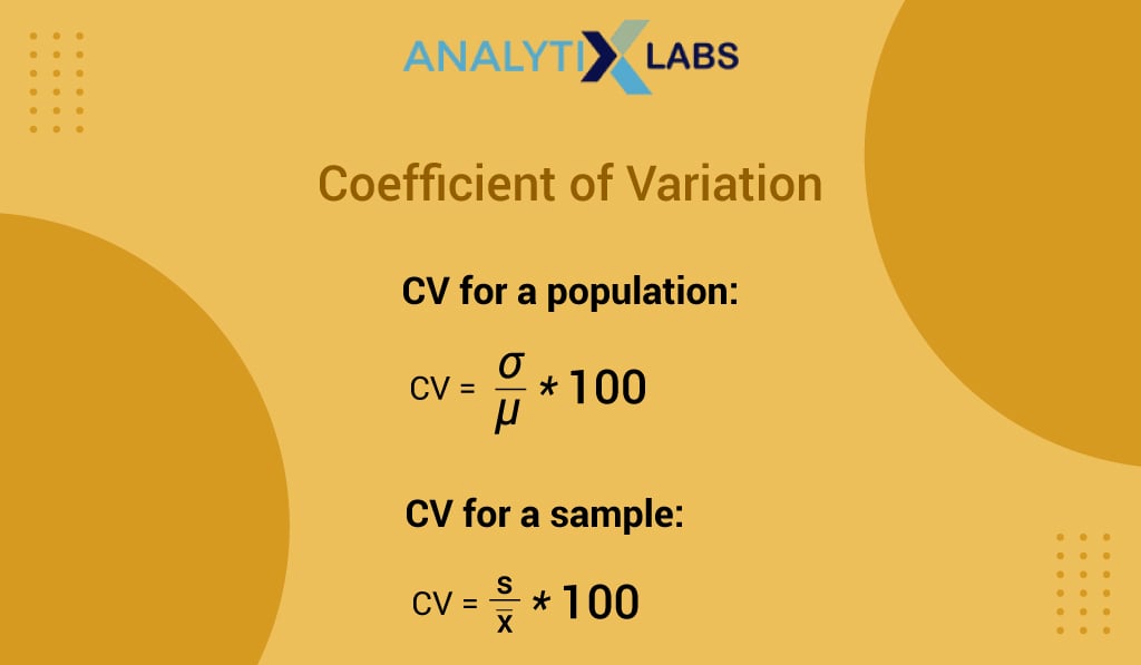
Let’s say we want to compare which of the two distributions are more variable, then we compare their respective coefficient of variation.

(4) Five-point Summary

Five-point summary is a measure that summarizes the center, location, and shape of the data. The five-point summary is:

1. Minimum value (the smallest observation in the data)
2. First Quartile (Q1)
3. Second Quartile (Median or Q2)
4. Third Quartile (Q3)
5. Maximum value (the largest observation in the data)

To create a five-point summary, the first step is to arrange the data in ascending order and then identify the smallest value, largest value, and the three quartiles (Q1, Q2, and Q3).

The five-point summary is visually also depicted in a graph called boxplot, which looks like:

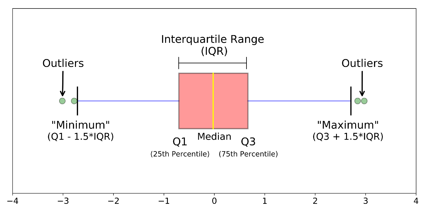
Image Source: Understanding Boxplots published on Towards Data Science

An additional step to creating a boxplot is to calculate the IQR i.e., the interquartile range. Boxplot is a very useful graphical summary that helps in identifying the outliers present in the data. Up until now, the measures we have seen are used to summarize the data for a single or one variable at a time. To understand and see the relationship between two variables we use the below measure. 

(5) Measure of Association between two variables

• Covariance

Covariance, as a descriptive measure, measures the strength of the linear relationship between two numerical variables.

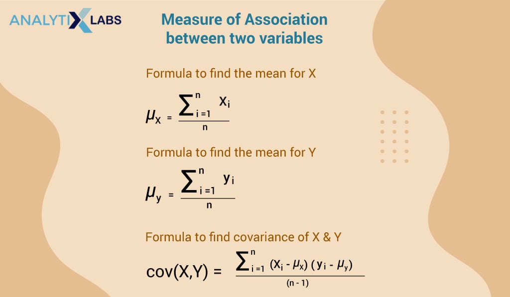
Covariance cannot tell whether the value indicates a strong or weak relationship because covariance can take any value and the value of the covariance depends on the units of measurement of the variables x and y. This is where the next measure, the correlation coefficient comes to aid us. 

• Correlation Coefficient

A measure of the relationship between the two variables that are not affected by the units of measurement is known as the correlation coefficient. What this measure tells us is the relative strength of a linear relationship between two variables that are numerical in nature. 

The correlation coefficient ranges from -1 to +1. Values closer to -1 or +1 indicate a strong linear relationship and values closer to zero indicate weaker relationships. Scatter plots are used to visually show the relationship between two numerical variables.

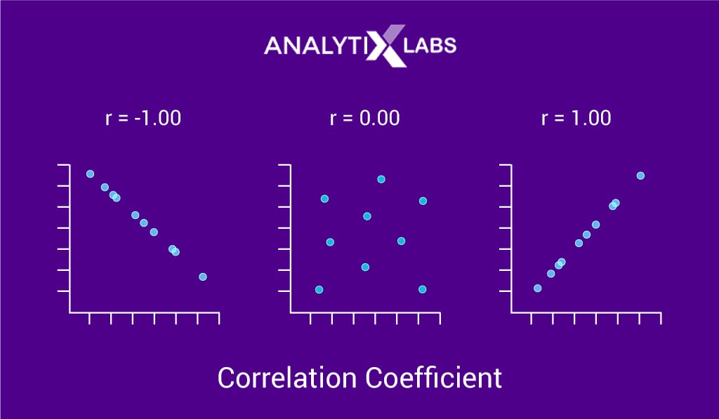
• Correlation coefficient of -1 indicates: a perfect negative relationship 
• Correlation coefficient of +1 indicates: a perfect positive relationship 

An important point to note is that the correlation provides a measure of a linear relationship and not causation. This means that a high correlation between two variables does not mean that a change in one variable will cause a change in another variable.

Inferential Statistics

We have been saying for some time now that by using inferential statistics we can make inferences about the population basis of the sample. Let’s understand what these two terms population and sample mean:

A population is the set of all elements of interest or observations in particular research or study. A sample is the subset of the population. The relationship between population and sample is depicted as below:

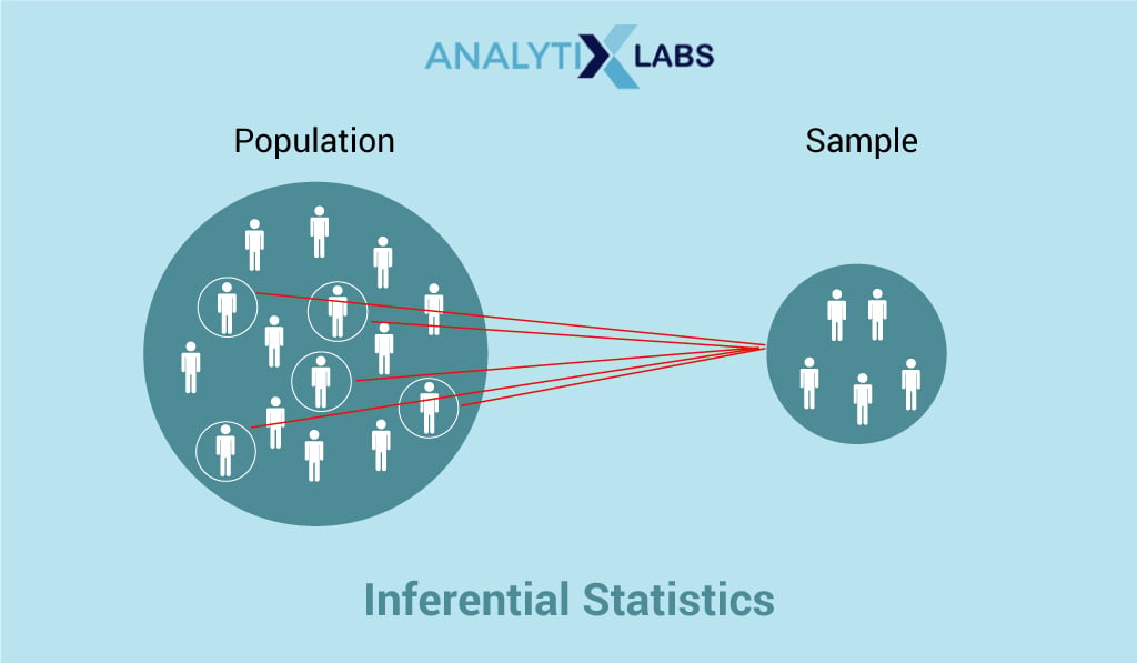
So, formally introducing the inferential research discipline: It consists of making inferences, forecasts, and estimates about the population, using the statistical features of a sample of data. Inferential Statistics is also known as Inductive statistics. 

When it comes to descriptive vs inferential statistics, the analysis is limited to the available data in descriptive statistics. However, that is not the case with inferential statistics. In inferential research, the analysis goes beyond the available data.

The sample chosen must represent the entire population so it must have all the important characteristics of the population. So, how do you think we can ensure that the sample accurately depicts the population? We can only make predictions to check this accuracy and when we predict anything, what result do we get? The output of predictions is probability.

Therefore, inferential statistics uses probability theory to ascertain if a sample is representative of the population or not. This process of checking for samples being a true representation of the population is obtained by sampling.

While performing any kind of sampling, certainly error occurs, this error is known as the sampling error. If there is a sampling error, then that means to some extent the sample is not accurately representing the population. 

Inferential statistics also considers the errors that come from sampling. Inferential data analysis is all about how much the sample differs from the population. It involves conducting more additional tests to determine if the sample is a true representation of the population. The ways of inferential statistics are: 

1. Estimating parameters
2. Hypothesis testing or Testing of the statistical hypothesis

Types of Inferential Statistics

The types of inferential statistics are as follows:

(1) Estimation of Parameters

In life, we tend to estimate almost everything. To reach from one place to another, we estimate the time it will take us to reach. We estimate the speed of the vehicle that is approaching while driving or crossing a road. We even estimate the time it will take to cook something. Using these estimations, we tune in the time or other adjustments needed to be made. In essence, estimation is part of our life and when we estimate anything, there is a possibility of error that needs to be accounted for.  

Now, in the statistical world, estimation is also of two kinds:

Point Estimation: A point estimate of a population parameter is a single value of a statistic. For example: taking the sample mean (i.e., a statistic from the sample data) to say something about the population mean (which is the population parameter) is an estimation.

A point estimator does not account for the possibility of error and therefore is not expected to provide the exact value of the population parameter, hence the need for interval estimation.

Interval Estimation: An interval estimate provides information about how close the point estimate (which is provided by the sample) is to the value of the population parameter. 

The interval estimate is defined by two numbers which are: point estimate +/ margin of error. The possibility of error in the statistical language is known as the margin of error.

(2) Hypothesis Testing

A hypothesis is an assumption or statement that is made in support of a finding or claim. This statement must be tested statistically for its viability. The inferential data analysis involves testing hypotheses or in other words, statements about the population based on the attributes of the sample. It is about determining the value of the underlying population parameter.

(3) Regression Analysis

Regression analysis is used for quantifying the association between variables. It is used to estimate how the variables are related, that is it mathematically shows how one variable changes with respect to another variable. To perform a regression analysis, we need to know the results of the hypothesis test.

How do Descriptive and Inferential Statistics treat data?

As we spoke at the beginning, the given captured raw data may not be organized nor have a structure to it; hence, it would not be easy to make sense of the data and visualize it. This is where the importance of descriptive statistics is visible as it encapsulates the data in a concise and meaningful manner along with an easy visual representation of the data enabling a simplified interpretation of the data. 

Let’s look at examples of inferential and descriptive statistics. It would help us understand how descriptive and inferential statistics are used for data. We are in charge of quality assurance with the responsibility of checking the quality of the manufactured products. We know that on average 50 products are defective. Our sample consists of these 50 products. Here, we have the following descriptive statistics for the 50 manufactured pieces in the sample:

• Sample mean
• Sample standard deviation
• Making a bar chart or boxplot
• Describing the shape of the sample probability distribution

Using the sample of these 50 products, we can make inferences about the entire population of 1000 products. So, the average product defective rate is a statistical central tendency measure (falling within the realms of descriptive statistics). The part to infer for all the 1000 products based on the sample of 50 products that are to generalize using the sample is Inferential Statistics. Also, based on this sample, we want to determine if we can predict whether the next new product will be defective or not. This can be estimated by conducting hypothesis testing. 

This shows that the primary factor to differentiate between descriptive and inferential statistics is what we do with the data 

Another point to note is how the measures of location and dispersion (that we saw under the descriptive statistics) are referred to differently for a population and sample. 

• When the measures are computed for population data, these are referred to as population parameters. 
• When the measures are computed for data from a sample, these are called sample statistics.

In inductive statistics, the sample statistic is referred to as the point estimator of the corresponding population parameter. 

Now, let’s see the difference between descriptive and inferential statistics.

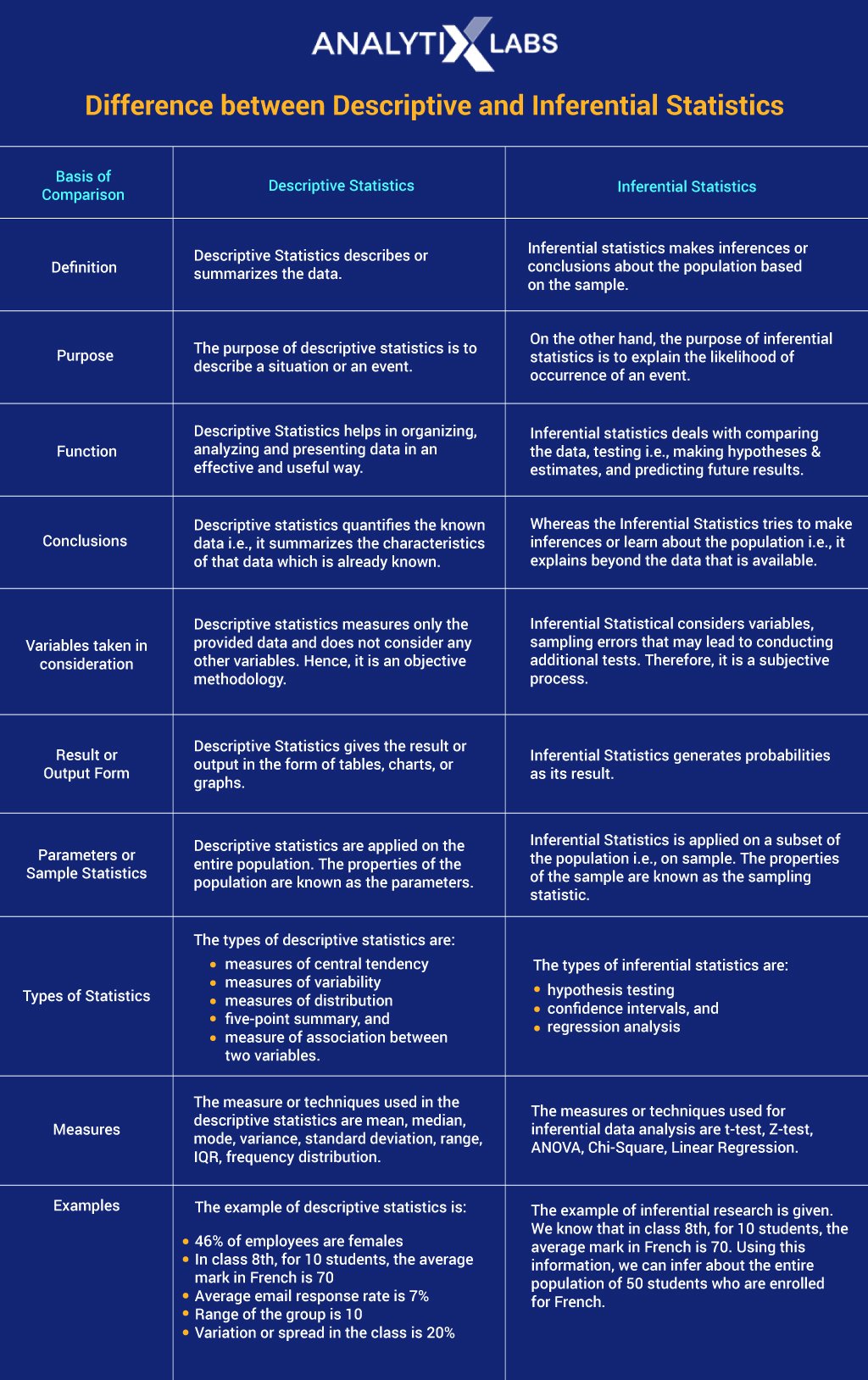
Difference between Descriptive and Inferential Statistics

The following table details descriptive vs inferential statistics as follows: 

Conclusion

Statistics and its branches are an integral part of any data cycle. Without statistical analysis, it’s very difficult to summarize and conclude anything about the data. The application of statistical analysis has its presence in almost all domains today including finance & accounting, marketing, research, IT, supply chain, and economics. 

The way of understanding data is using the primary branches of Statistics: descriptive and inferential statistics. Descriptive Statistics describes the data whereas inferential statistics make inferences or generalize the population using the sample. In a way, descriptive statistics can be seen as an objective process whereas inferential statistics is more subjective as it involves generalizing and estimates about the population using the sample. The descriptive and inferential statistics form the backbone of the data analysis. I hope this blog was helpful to understand the subdivisions of Applied statistics and the difference between descriptive and inferential statistics. 

Additionally you may like to read: 

• Understanding Perceptron: The founding element of Neural Networks
• How data compression technique helps in data representation?
• Understanding the basics of veracity in big data
• Understanding data structures: Types and applications
• What is data wrangling in machine learning