How are types of data related to data structures?

Although the primitive data structures are the same as that of the data types, there are differences between the two which are listed below: Data Type Data Structure Definition Data type describes the characteristics of the data. It classifies the data based on its nature or type. A data structure is a cluster or group which holds or stores the different types of data. It is a method to collect, store and organize the data to perform operations on these data efficiently. Storage Data types do not store the values as it only reflects the type of the data. Data structures hold the data, the types of data, and their values in a single object, which can be used for the entire program. Implementation The implementation of data types is abstract, meaning it depends on the given programming language. It is done from the end user’s perspective where the user does not need to know how the implementation will happen. On the other hand, data structures have concrete implementation and are used within an algorithm. Assignment The values are directly assigned to the data type variables. Here, the data is designated to a data structure object via algorithms and operations such as push, pop. Performance & complexity Data types do not have any complexity both in management and time. Data structures need management and are complex time-wise as well as these contain multiple primitive data types. It involves organizing in memory terms, then accessing, manipulating, and executing the values via defined logic. Example Int, float, str, char Arrays, Linked Lists, Stacks, Queues, Trees, Graphs, Hash tables, Heaps

What are the applications of different types of data structures?

The applications of the types of the data structure are as follows:

(1) What are the advantages of data structures?

The advantages are as follows: Data structures are an efficient and safe way to store data on devices and hard disks. It is also convenient to retrieve data from these devices. It allows for easier and more effective processing of both large and small data. It helps in optimizing the time for operations including storage, retrieval, and processing. The data stored on the structure is safe and secure and does not get lost. Data structures are reusable. It can be used by multiple client programs.

(2) How do you choose the right data structure?

A four-step methodology selects the right data structure that considers and answers some of the basic concerns. The steps are as follows: Relevance of the data structure to the business problem: The objective of any program is to solve a business problem and hence, the data structure chosen must be suitable and appropriate to the problem at hand and not based only on the familiarity with the data structure. This has another consequence of resulting in a slow program and later needs to be improved. Operations to be performed on the data: The next part is choosing the data structure to analyze the problem to understand what basic operations and functions are needed and must be supported by the program. Some of the operations that are important for a program are: Insertion of data in the data structure Delete the data items Searching for specific values within the data Checking the computational complexity: Along with the functional use and appropriateness of the data structure, must take into account the threshold of the computational performance. A complex program could need improvements to achieve the performance goals wherein a simpler program and design could be a sufficient solution. Implementation: Select the data structures that meet the requirements.

(4) Where are data structures applied?

Data structures are applied in – Compiler Design Operating System Database Management System (DBMS) Database Design and Management Numerical and Statistical analysis Simulation Machine Learning Artificial Intelligence Image & Speech Processing Graphics Blockchain Cryptography

(5) Is a pointer a data structure?

No, a pointer is not a data structure. It is a type. Pointers store the address of another variable or its memory location. They don’t hold any data value. These are used for reference to other values, therefore are known as reference data types. For example, a string variable saves the name of a person, and the string printer simply refers or points to the address of that string variable.

Understanding Data Structures: Types and Applications

One of the fundamental topics of Computer Science and Software Engineering that have varied applications and use in Data Science is Data Structures. Different types of data structures are the building block of any program or software, and it is a core construct to build any of the programs. A program is built using algorithms and data structures that are the natural, logical progression of the data, the bread and butter of Data Science.

You have to pay heed to data structures to ensure that our programs and codes run effectively and orderly for the chosen data structure. Each data structure employs different operations. When you think about the future of data science and its implications, you need to learn about applying the algorithms that work well and fastest on the given data structure. This article will cover the data structures, the types of trees in the data structure, their types, their applications, and how the types of data are related to the data structures.

You may also want to read: What Is the Difference Between Data Science Vs. Computer Science?

Data Structure: Definition

A data structure is a technique to systematically store data so that the data can be easily and effectively created, accessed, and managed. This system collects data values, how they are related to each other, and the operations that can be applied to the data.

For example, let’s say we have data with values such as Richard Branson, 70, United Kingdom. This data is composed of different data types: string and integer. The name – Richard Branson, and location – United Kingdom, are of string data type, and age 70 is of integer. This data can be organized in entrepreneurs’ data with their name, location, and age. This collected data can be further stored in a database as a data structure and used for future operations.

In other words, we see data structure as a channel or vehicle to work with the data. It is a method to collect, store and organize data for later use. There are various data structures available using their respective utility and function. Each of the data structures offers a specific way to organize data so that it can be accessed most efficiently.

Now, let’s take a look at the different types of data structures.

Types of Data Structures

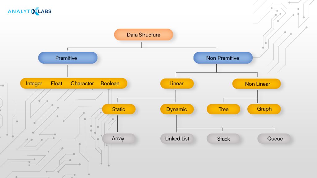
Data structures are grouped based on the type of operations required to perform. The two broad types of the data structure are:

Primitive data structures i.e. built-in data structures
Non-primitive data structures or the derived data structures

The Non-Primitive data structure can be further categorized into Linear and Nonlinear data structures, which can be further classified based on how the data is stored. The types of trees in the data structure flow are as follows:

types of data structure

Primitive Data Structures

Primitive data structures are the basic integral structures that are supported at the machine level. These structures have predefined specifications and characteristics. These are also known as built-in types and have in-built support from the programming language. These can be used to create on-primitive data structures. Examples are:

Integer: Integers are whole numbers that can store zero, positive or negative values. Different programming languages and databases can store different-sized integers with varied ranges of values.
Real(float): Real or float numbers are decimal numbers. When you require maximum precision, Float is used. Single precision is a 32-bit floating-point number and double precision is a 64-bit floating number.
Characters: Characters represent letters, symbols, and even whitespace. A string is an array of characters.
Booleans: stores the logical values true or false.

Non-primitive Data Structures

Non-primitive data structures are derived from primitive data structures and are more complicated. These rely on primitive structures and focus on grouping the homogenous or heterogenous values in a form. Therefore, these are also known as the derived types.

Non-primitive structures are usually more preferred as these are more flexible compared to primitive’s ones. The user can construct its non-primitive structure considering the operations to perform.

Non-Primitive Data Structures can again be classified into two categories:

Linear Data Structures
Non-Linear Data Structures

Linear Data Structures

In a linear data structure, the values are stored sequentially or linearly. The values are arranged in a single level where each value is linked to the previous and the next value. It is easy to implement as is lineally organized and hence can access each value in a single run.

There is one more layer of the subdivision. Linear data structures can be segmented as static and dynamic. Arrays are an example of static linear data structure and dynamic linear data structures consist of Linked Lists, Stacks, and Queues.

Static linear data structure:

The static linear data structures are the ones where the sizes and the associated memory locations are fixed at the compilation time. Arrays are static.

Arrays:

An Array is defined as “an ordered series or arrangement”, and it is the collection of homogeneous elements with consecutive memory locations.

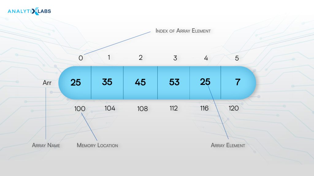
array static linear data structure

The array has two important terms: elements and indexes.

Elements: each of the values stored in an array is called an element, and
Indexes: The unique value or key that is used to identify the element is called the index. An index is the position of the array element and is not the memory location. It usually starts with 0.

Here, the array length is 6, meaning this array stores six values or elements. In Python, we can retrieve the element with the index of 2 as Arr[2], giving 45.

The array elements usually share the same variable name; however, each element has its unique index or key, which is also known as the subscript. The elements can be easily randomly retrieved using their index number in this simplest data structure. Arrays can be one-dimensional, two-dimensional, or multidimensional.

types of array

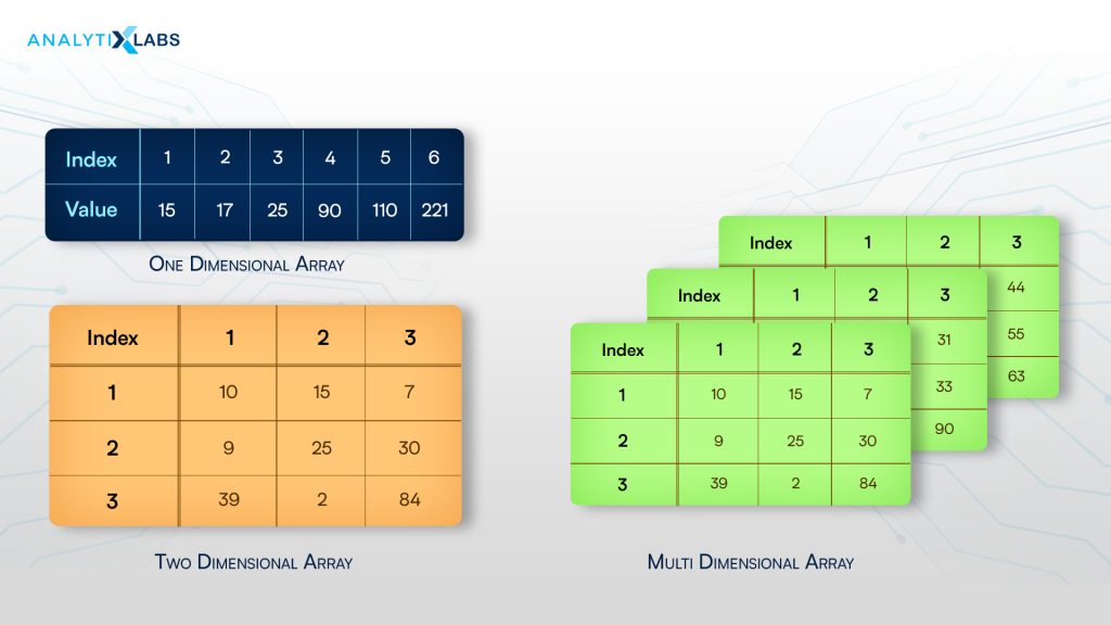
The purpose of an array is to organize the data so that the related set of values can be easily sorted or searched. Arrays can have fixed or flexible lengths. We can store a group of integers, floating-point numbers, strings, or even other arrays within an array.

These are static because they have fixed memory allocation meaning once a memory space is assigned to a value, it cannot be modified on a runtime basis. The operations of insertion and deletion are complex because the elements are stored in adjacent memory allocations.

Arrays are the most fundamental static linear data structure and are essential to knowing how to build dynamic linear data structures. It is also used to apply to vectors and matrices.

Dynamic linear data structure:

The dynamic linear data structures can expand or reduce depending upon the program’s need and its execution. Additionally, the associated memory locations are changeable, and examples are Linked Lists, Stacks, and Queues.

(1) Linked Lists:

A linked list is a linear non-primitive data structure that holds the collections of elements in a linear order. Here, these elements or nodes are linked together as a chain or sequence and stored in non-contiguous memory locations. Linked lists comprise two main parts: the element or the data itself and the pointer or the address referencing the adjacent node. The start of the linked list is labeled as the head and the end of the linked list is marked as the tail or the null.

linked lists

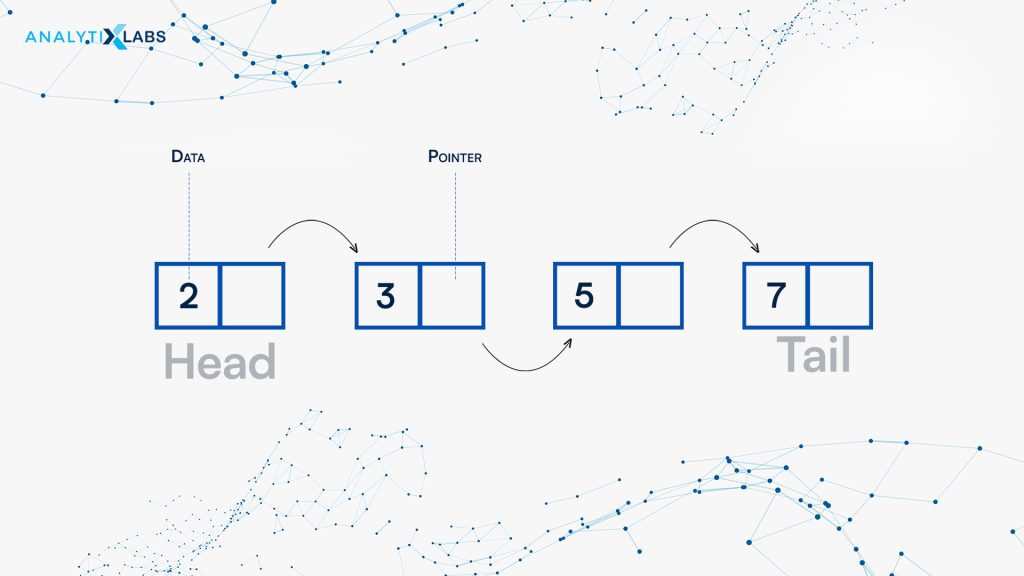
There are three types of linked lists:

Singly-linked list: Elements can navigate only in the forward direction.
Doubly-linked list: The elements can navigate both in the forward and backward directions.
Circular-linked list: Elements navigate in a circular chain as the last element holds the address of the first element.

(2) Stacks

The stack linear data structure is exactly like a real physical pile of things arranged one on top of another, and it is an ordered list of elements of similar data types. The structure stores and retrieves data on the LIFO basis i.e. Last in First out.The insertion and the deletion of the elements in a stack happen from the top of the stack and the most recently inserted element gets deleted first. A stack has three basic operations:

Push: Insert the element on the top of the stack
Pop: Remove the top-most element from the stack
Pip: Display the content of the stack

This is illustrated below:

stacks dynamic ata structure

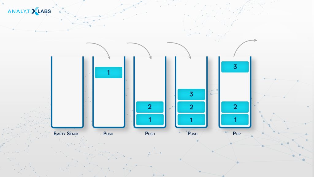
A stack is in an overflow state when it is completely full and is in an underflow state when it is empty. The stack data structure is an abstract data type (ADT) with a predefined or bounded capacity, meaning the stack can hold elements of a limited size.

(3) Queues

Like stacks, are also abstract data structures and are an ordered list of elements having similar data types. Queues follow the FIFO method i.e First in First Out for storing and retrieval of the elements.

Unlike stacks, queues are open from both ends. It works exactly how a real queue works. Consider a ticket counter or queue for parking, where a person or vehicle that enters, leaves first. The elements are inserted only from one end, called the Rear (back or the tail) and the elements are removed from the other end, which is the front of the queue.

En-queue: Process of inserting the element into the queue.
De-queue: Process of removing the element from the queue.

queues dynamic data structure

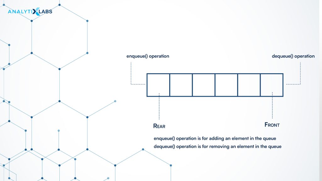
Both stacks and queues can be implemented via arrays, linked lists, pointers, and structures.

Non-linear Data Structures

In a nonlinear data structure, the data values are arranged in a non-sequential manner and at multiple levels. In this nonlinear arrangement, each of the values is connected to two or more two values. It needs multiple runs to traverse as the values cannot be accessed in one run. Examples of the nonlinear data structure are Trees and Graphs.

(1) Graphs

Graphs are defined as – A pictorial representation of a set of elements that are connected by links. Like, arrays, graphs have two components: vertices or nodes and edges.

Vertices or Nodes: The elements in a graph are known as Nodes or vertices.
Edges: Links that connect the vertices are called Edges. A set of edges is the connector between these vertices.

The number of vertices of nodes in the order of the graph and the number of edges define the size of the graph. The nodes having the same edge or the connector are said to be the adjacent or neighboring nodes.

A graph data structure represents a network as it has a cycle. This nonlinear non-primitive data structure can be perceived as a cyclic tree where the nodes do not have a parent-child relationship and are more complex. There are different types of graphs :

Directed Graph: In a directed graph, all the edges have directions from where the connection starts and ends.
Undirected Graph: The edges do not have any directions associated with them in the undirected graph.

types of graphs

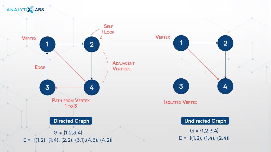
In the above image of the directed graph on the left side, nodes 1 and 4 clearly indicate the direction starting from node 1 and reaching node 4. And on the right side image of the undirected graph, the edges do not have any direction indicators. Here, the connections can traverse from vertex 1 to vertex 4 or from vertex 4 to vertex 1.

A self-loop is having the edges from the vertex to itself, and an isolated is where the node is not connected to any other node in the graph.

(2) Trees

Trees are nonlinear multilevel data structures having a hierarchical relationship among the elements. These elements or the nodes are linked and form a parent-child relationship. The nodes have The tree data structure is graphically represented below:

tree structure

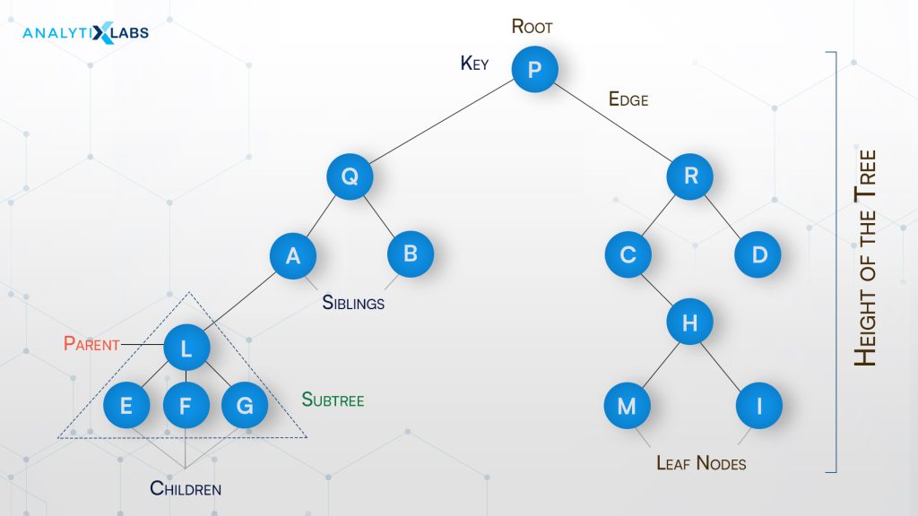
The tree starts with a root node which branches out further into various child nodes. These child nodes are also known as subnodes. Each node can have at maximum only one parent apart from the starting root node. The last node that can not be subdivided anymore is known as the leaf node.

The height of the tree is equivalent to the number of levels of the tree. Similar to the graphs, the trees have pointers that point the subnodes to the main node. These can be called the edges or references. However, unlike graphs, in trees, there is only one possible downward path from the parent to the child node and not vice-versa and no edge is duplicated.

There are various types of trees available. Some of the common tree structures are:

Binary Trees
Binary Search Trees
Heaps
Trees
Trie
B-Trees
AVL Trees

For more visual learning, you can follow the explanation by Knowledge Hub –