What is Clustering in Machine Learning: Types and Methods

Before we get into the types of clustering, here’s what we are dealing with.

Many things around us can be categorized as “this and that” or to be less vague and more specific. We have groupings that could be binary or groups that can be more than two, like a type of pizza base or type of car that you might want to purchase. The choices are always clear – or, how the technical lingo wants to put it – predefined groups and the process of predicting that is an important process in the Data Science stack called Classification.

But what if we bring into play a quest where we don’t have pre-defined choices initially. Rather, we derive those choices! Choices that are based on hidden patterns, underlying similarities between the constituent variables, salient features from the data, etc. This process is known as Clustering in Machine Learning or Cluster Analysis, where we group the data together into an unknown number of groups and later use that information for further business processes.

Clustering aims to discover meaningful structure, explaining the underlying process, descriptive attributes, and groupings in the selected set of examples. The categorization can use different approaches and algorithms depending on the available data and the required sets.

You may also like to read: What is Machine Learning?

What is Clustering?

Clustering or Cluster analysis is the method of grouping the entities based on similarities. Defined as an unsupervised learning problem that aims to make training data with a given set of inputs but without any target values. It is the process of finding similar structures in a set of unlabeled data to make it more understandable and manipulative.

It reveals subgroups in the available heterogeneous datasets such that every individual cluster has greater homogeneity than the whole. In simpler words, these clusters are groups of like objects that differ from the objects in other clusters.

In clustering, the machine learns the attributes and trends by itself without any provided input-output mapping. The clustering algorithms extract patterns and inferences from the type of data objects and then make discrete classes of clustering them suitably.

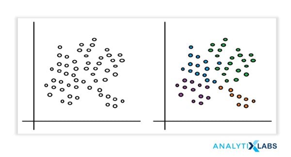
Types of Clustering Methods

Clustering helps in performing surface-level analyses of the unstructured data. The cluster formation depends upon different parameters like shortest distance, graphs, and density of the data points. Grouping into clusters is conducted by finding the measure of similarity between the objects based on some metric called the similarity measure. It is easier to find similarity measures in a lesser number of features. Creating similarity measures becomes a complex process as the number of features increases. Different types of clustering approaches in data mining use different methods to group the data from the datasets. This section describes the clustering approaches.

The various types of clustering are:

1. Connectivity-based Clustering (Hierarchical clustering)
2. Centroids-based Clustering (Partitioning methods)     
3. Distribution-based Clustering
4. Density-based Clustering (Model-based methods)
5. Fuzzy Clustering
6. Constraint-based (Supervised Clustering)

1. Connectivity-based Clustering (Hierarchical Clustering)

Hierarchical clustering, also known as connectivity-based clustering, is based on the principle that every object is connected to its neighbors depending on their proximity distance (degree of relationship). The clusters are represented in extensive hierarchical structures separated by a maximum distance required to connect the cluster parts. The clusters are represented as Dendrograms, where X-axis represents the objects that do not merge while Y-axis is the distance at which clusters merge. The similar data objects have minimal distance falling in the same cluster, and the dissimilar data objects are placed farther in the hierarchy. Mapped data objects correspond to a Cluster amid discrete qualities concerning the multidimensional scaling, quantitative relationships among data variables, or cross-tabulation in some aspects. The hierarchical clustering may vary in the data flow chosen in the following categories.

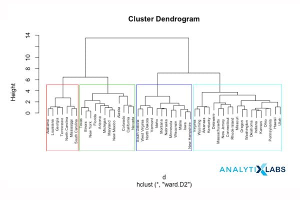
1.1 Divisive Approach

This approach of hierarchical clustering follows a top-down approach where we consider that all the data points belong to one large cluster and try to divide the data into smaller groups based on a termination logic or a point beyond which there will be no further division of data points. This termination logic can be based on the minimum sum of squares of error inside a cluster, or for categorical data, the metric can be the GINI coefficient inside a cluster.

Hence, iteratively, we are splitting the data, which was once grouped as a single large cluster, into “n” number of smaller clusters to which the data points now belong.

It must be taken into account that this algorithm is highly “rigid” when splitting the clusters – meaning, once a clustering is done inside a loop, there is no way that the task can be undone.

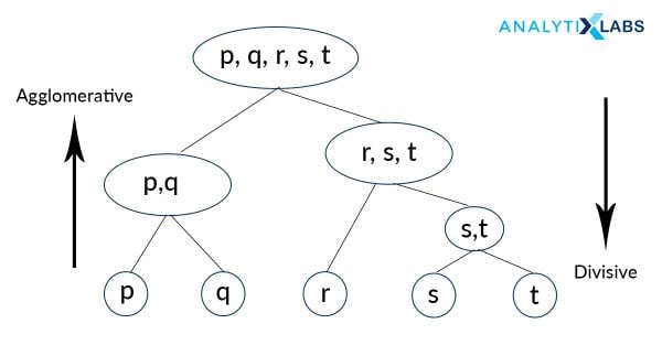
1.2 Agglomerative Approach

Agglomerative is quite the contrary to Divisive, where all the “N” data points are considered to be a single member of “N” clusters that the data is comprised into. We iteratively combine these numerous “N” clusters to a fewer number of clusters, let’s say “k” clusters, and hence assign the data points to each of these clusters accordingly. This approach is a bottom-up one, and also uses a termination logic in combining the clusters. This logic can be a number-based criterion (no more clusters beyond this point) or a distance criterion (clusters should not be too far apart to be merged) or a variance criterion (increase in the variance of the cluster being merged should not exceed a threshold, Ward Method)

2. Centroid-based or Partition Clustering

Centroid-based clustering is the easiest of all the clustering types in data mining. It works on the closeness of the data points to the chosen central value. The datasets are divided into a given number of clusters, and a vector of values references every cluster. The input data variable is compared to the vector value and enters the cluster with minimal difference.

Pre-defining the number of clusters at the initial stage is the most crucial yet most complicated stage for the clustering approach. Despite the drawback, it is a vastly used clustering approach for surfacing and optimizing large datasets. The K-Means algorithm lies in this category.

These groups of clustering methods iteratively measure the distance between the clusters and the characteristic centroids using various distance metrics. These are either Euclidian distance, Manhattan Distance or Minkowski Distance.

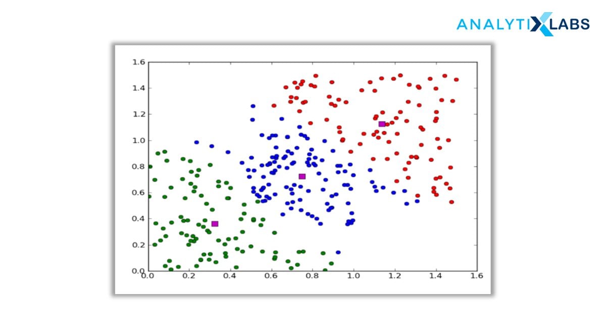
The major setback here is that we should either intuitively or scientifically (Elbow Method) define the number of clusters, “k”, to begin the iteration of any clustering machine learning algorithm to start assigning the data points.

Also, owing to their simplicity in implementation and also interpretation, these algorithms have wide application areas viz., market segmentation, customer segmentation, text topic retrieval, image segmentation, etc.

3. Density-based Clustering (Model-based Methods)

The first two methods discussed above depend on a distance (similarity/proximity) metric. The very definition of a cluster is based on this metric.

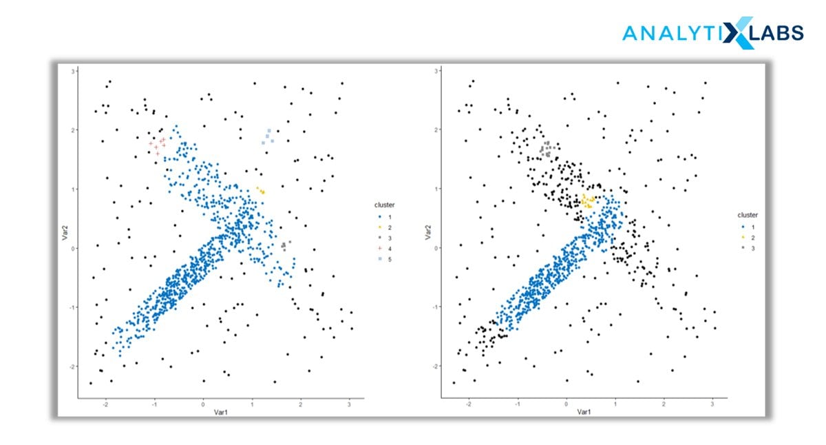
Density-based clustering method considers density ahead of distance. Data is clustered by regions of high concentrations of data objects bounded by areas of low concentrations of data objects. The clusters formed are grouped as a maximal set of connected data points.

The clusters formed vary in arbitrary shapes and sizes and contain a maximum degree of homogeneity due to similar density. This clustering approach includes the noise and outliers in the datasets effectively.

When performing most of the clustering, we take two major assumptions: the data is devoid of any noise and the shape of the cluster so formed is purely geometrical (circular or elliptical).

The fact is, data always has some extent of inconsistency (noise) which cannot be ignored. Added to that, we must not limit ourselves to a fixed attribute shape. It is desirable to have arbitrary shapes to not to ignore any data points. These are the areas where density-based algorithms have proven their worth!

4. Distribution-Based Clustering

Until now, the clustering techniques as we know them are based on either proximity (similarity/distance) or composition (density). There is a family of clustering algorithms that take a totally different metric into consideration – probability.

Distribution-based clustering creates and groups data points based on their likely hood of belonging to the same probability distribution (Gaussian, Binomial, etc.) in the data.

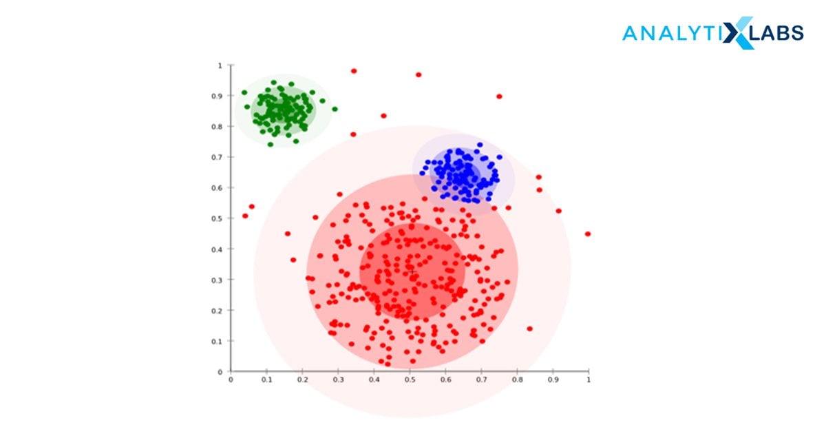
It is a probability-based distribution that uses statistical distributions to cluster the data objects. The cluster includes data objects that have a higher probability to be in it. Each cluster has a central point, the higher the distance of the data point from the central point, the lesser will be its probability to get included in the cluster.

A major drawback of density and boundary-based approaches is in specifying the clusters apriori to some of the algorithms and mostly the definition of the shape of the clusters for most of the algorithms. There is at least one tuning or hyper-parameter which needs to be selected and not only that is trivial but also any inconsistency in that would lead to unwanted results.

Distribution-based clustering has a vivid advantage over the proximity and centroid-based clustering methods in terms of flexibility, correctness, and shape of the clusters formed. The major problem however is that these clustering methods work well only with synthetic or simulated data or with data where most of the data points most certainly belong to a predefined distribution, if not, the results will overfit.

5. Fuzzy Clustering

Fuzzy clustering generalizes the partition-based clustering method by allowing a data object to be a part of more than one cluster. The process uses a weighted centroid based on the spatial probabilities.

The steps include initialization, iteration, and termination, generating clusters optimally analyzed as probabilistic distributions instead of a hard assignment of labels.

The algorithm works by assigning membership values to all the data points linked to each cluster center. It is computed from a distance between the cluster center and the data point. If the membership value of the object is closer to the cluster center, it has a high probability of being in the specific cluster.

At the end iteration, associated values of membership and cluster centers are reorganized. Fuzzy clustering handles the situations where data points are somewhat in between the cluster centers or ambiguous. This is done by choosing the probability rather than distance.

6. Constraint-based (Supervised Clustering)

The clustering process, in general, is based on the approach that the data can be divided into an optimal number of “unknown” groups. The underlying stages of all the clustering algorithms are to find those hidden patterns and similarities without intervention or predefined conditions. However, in certain business scenarios, we might be required to partition the data based on certain constraints. Here is where a supervised version of clustering machine learning techniques comes into play.

A constraint is defined as the desired properties of the clustering results or a user’s expectation of the clusters so formed – this can be in terms of a fixed number of clusters, the cluster size, or important dimensions (variables) that are required for the clustering process.

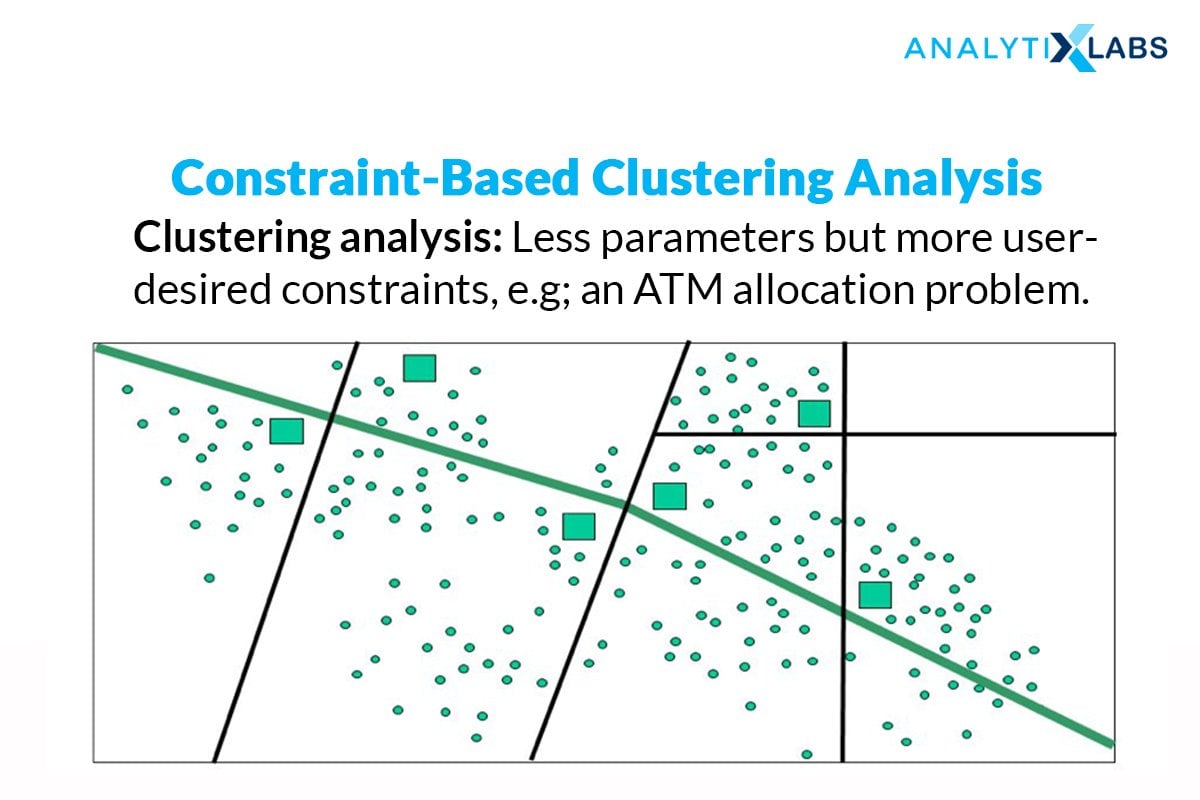
Usually, tree-based, Classification machine learning algorithms like Decision Trees, Random Forest, Gradient Boosting, etc. are made use of to attain constraint-based clustering. A tree is constructed by splitting without the interference of the constraints or clustering labels. Then, the leaf nodes of the tree are combined together to form the clusters while incorporating the constraints and using suitable algorithms.

Types of Clustering Algorithms 

Clustering algorithms are used in exploring data, anomaly detection, finding outliers, or detecting patterns in the data. Clustering is an unsupervised learning technique like neural network and reinforcement learning. The available data is highly unstructured, heterogeneous, and contains noise. So the choice of algorithm depends upon how the data looks like. A suitable clustering algorithm helps in finding valuable insights for the industry. Let’s explore the different types of clustering in machine learning in detail.

1. · K-Means clustering
2. Mini batch K-Means clustering algorithm
3. Mean Shift
4. Divisive Hierarchical Clustering
5. Hierarchical Agglomerative clustering
6. Gaussian Mixture Model
7. DBSCAN
8. OPTICS
9. BIRCH Algorithm

1. K-Means clustering

K-Means is a partition-based clustering technique that uses the distance between the Euclidean distances between the points as a criterion for cluster formation. Assuming there are ‘n’ numbers of data objects, K-Means groups them into a predetermined ‘k’ number of clusters.

Each cluster has a cluster center allocated and each of them is placed at farther distances. Every incoming data point gets placed in the cluster with the closest cluster center. This process is repeated until all the data points get assigned to any cluster. Once all the data points are covered the cluster centers or centroids are recalculated.

After having these ‘k’ new centroids, a new grouping is done between the nearest new centroid and the same data set points. Iteratively, there may be a change in the k centroid values and their location this loop continues until the cluster centers do not change or in other words, centroids do not move anymore. The algorithm aims to minimize the objective function

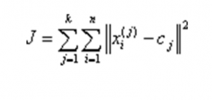
Where

, is the chosen distance between cluster center CJ and data point XI

The correct value of K can be chosen using the Silhouette method and Elbow method. The Silhouette method calculates the distance using the mean intra-cluster distance along with an average of the closest cluster distance for each data point. While the Elbow method uses the sum of squared data points and computes the average distance.

Implementation: K-Means clustering algorithm

•         Select ‘k’ number of clusters and centroids for each cluster.
•         Shuffle the data points in the dataset and initialize the selected centroid.
•         Assign the clusters to the data points without replacement.
•         Create new centroids by calculating the mean value of the samples.
•         Reinitialize the cluster centers until there is no change in the clusters.

2. Mean Shift Clustering algorithm

Mean shift clustering is a nonparametric, simple, and flexible clustering technique.  It is based upon a method to estimate the essential distribution for a given dataset known as kernel density estimation. The basic principle of the algorithm is to assign the data points to the specified clusters recursively by shifting points towards the peak or highest density of data points. It is used in the image segmentation process.

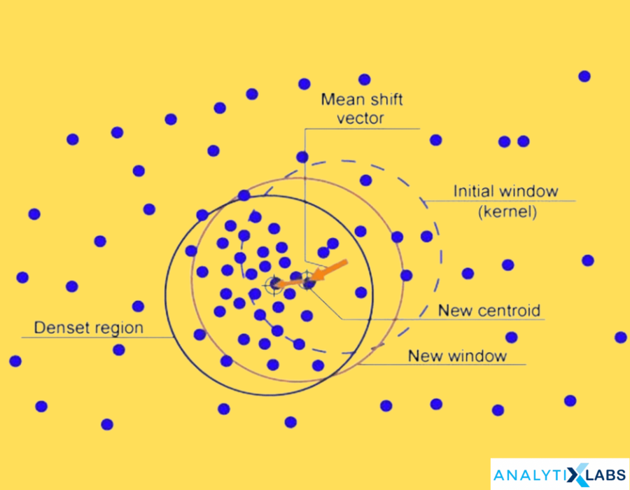
Algorithm:

Ø  Step 1 – Creating a cluster for every data point

Ø  Step 2 – Computation of the centroids

Ø  Step 3 – Update the location of the new centroids

Ø  Step 4 – Moving the data points to higher density regions, iteratively.

Ø  Step 5 – Terminates when the centroids reach a position where they don’t move further.

3. Gaussian Mixture Model

The gaussian mixture model (GMM) is a distribution-based clustering technique. It is based on the assumption that the data comprises Gaussian distributions. It is a statistical inference clustering technique. The probability of a point being a part of a cluster is inversely dependent on distance, as the distance from distribution increases, the probability of a point belonging to the cluster decreases. The GM model trains the dataset and assumes a cluster for every object in the dataset. Later, a scatter plot is created with data points with different colors assigned to each cluster.

GMM determines probabilities and allocates them to data points in the ‘K’ number of clusters. Each of which has three parameters: Mean, Covariance and mixing probability. To compute these parameters GMM uses the Expectation Maximization technique.

Source: Alexander Ihler’s YouTube channel

The optimization function initiates the randomly selected Gaussian parameters and checks whether the hypothesis belongs to the chosen cluster. Then, the maximization step updates the parameters to fit the points into the cluster. The algorithm aims at raising the likelihood of the data sample associated with the cluster distribution which states that the cluster distributions have high peaks (closely connected cluster data) and the mixture model captures the dominant pattern data objects by component distribution).

4. DBSCAN

DBSCAN – Density-Based Spatial Clustering of Applications with Noise identifies discrete groups in data. The algorithm aims to cluster the data as contiguous regions having high point density. Each cluster is separated from the others by points of low density. In simpler words, the cluster covers the data points that fit the density criteria which is the minimum number of data objects in a given radius.

Terms used in DBSCAN:

•         Core: Point having least points within the distance from itself
•         Border: Point having at least one core point from a given distance.
•         Noise: Having less than m points within a given distance. This point is neither the core nor the border.
•         minPts: A threshold value of a minimum number of points that considers the cluster to be dense.
•         eps ε: The distance measure used to put the points in the region of any other data point.
•         Reachability: Density distribution identifying whether a point is reachable from other points if it lies at a distance eps from it.
•         Connectivity: Transitivity-based chaining approach that establishes the location of any point in a specified cluster.

For implementing DBSCAN, we first begin with defining two important parameters – a radius parameter eps (ϵ) and a minimum number of points within the radius (m).

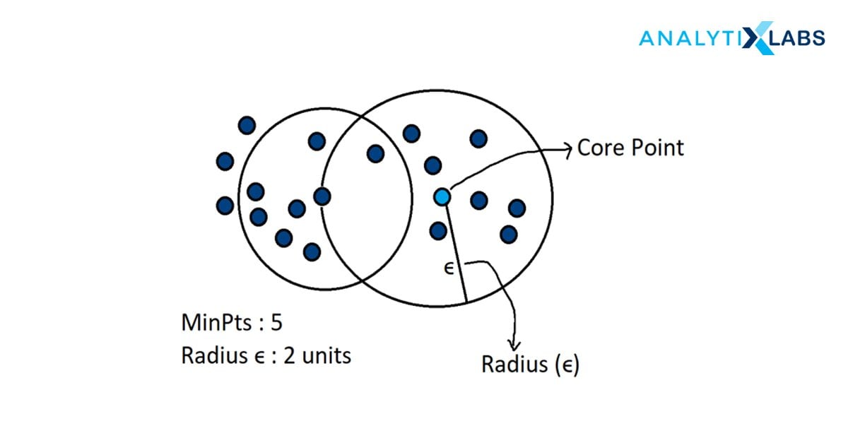
• The algorithm starts with a random data point that has not been accessed before and its neighborhood is marked according to ϵ.
• If this contains all the m minimum points, then cluster formation begins – hence marking it as “visited” – if not, then it is labeled as “noise” for that iteration, which can get changed later.

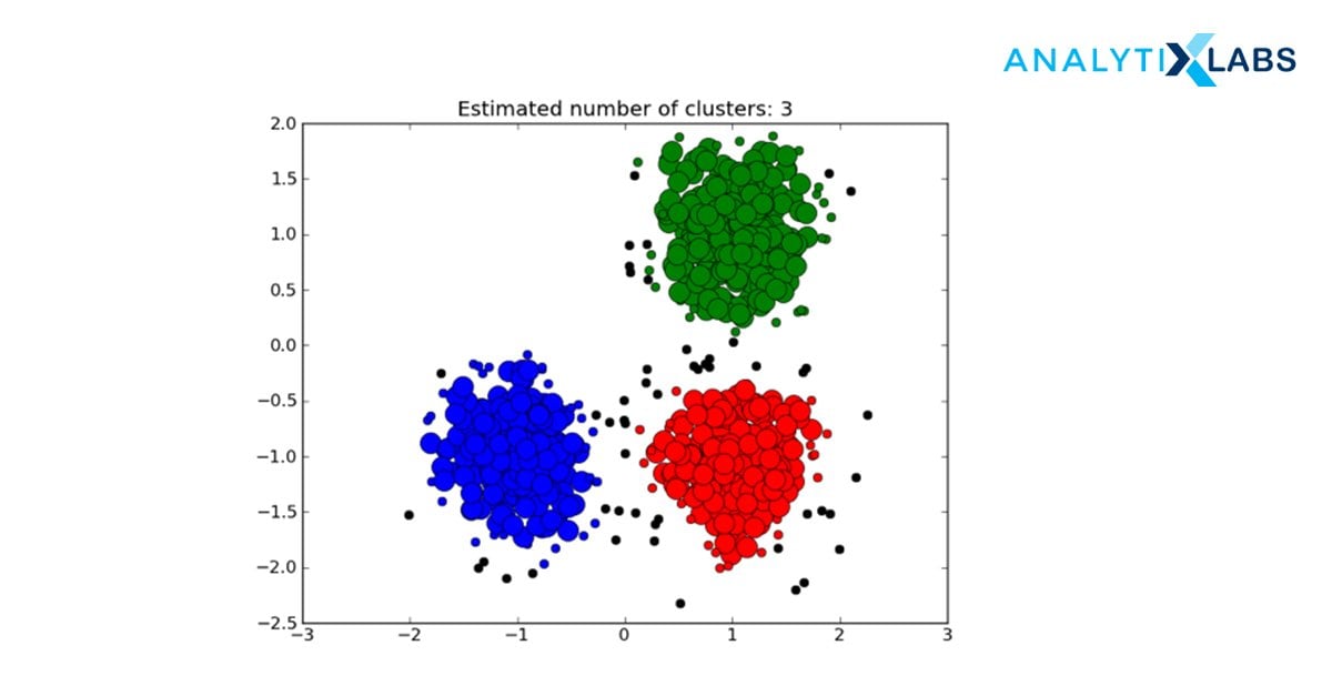
• If a next data point belongs to this cluster, then subsequently the ϵ neighborhood now around this point becomes a part of the cluster formed in the previous step. This step is repeated until there are no more data points that can follow Density Reachability and Density Connectivity.
• Once this loop is exited, it moves to the next “unvisited” data point and creates further clusters or noise
• The algorithm converges when there are no more unvisited data points remain.

Steps:

• Starting from a random point, all the points in the space are visited.
• The neighborhood is computed using distance epsilon ε to determine if it is a core point or an outlier. If it’s a core point cluster is made around the point.
• Cluster expansion is done by adding the reachable points in the proximity radius.
•  Repeating the steps until all points join the clusters or are labeled as outliers.

5. BIRCH Algorithm

Balanced Iterative Reducing and Clustering using Hierarchies, or BIRCH is a clustering technique used for very large datasets. A fast algorithm that scans the entire dataset in a single pass. It is dedicated to solving the issues of large dataset clustering by focusing on densely occupied spaces and creating a precise summary.

BIRCH fits in with any provided amount of memory and minimizes the I/O complexity. The algorithm only works to process metric attributes, which means the one with no categorical variables or the attribute whose value can be represented by explicit coordinates in a Euclidean space. The main parameters of the algorithm are the CR tree and the threshold.  

• CF tree: The clustering Feature tree is a tree in which each leaf node consists of a sub-cluster. Each entry in a CF tree holds a pointer to a child node. The CF entry is made up of the sum of CF entries in the child nodes. 
• Threshold: A maximum number of entries in each leaf node

Steps of BIRCH Algorithm

Step 1- Building the Clustering feature (CF) Tree: Building small and dense regions from the large datasets. Optionally, in phase 2 condensing the CF tree into further small CF.

Step 2 – Global clustering: Applying clustering algorithm to leaf nodes of the CF tree.

Step 3 – Refining the clusters, if required.

Applications of Clustering

Clustering is applied in various fields to prepare the data for various machine learning processes. Some of the applications of clustering are as follows.

1. Market segmentation: Businesses need to segment their market into smaller groups to understand the target audience. Clustering groups the like-minded people considering the neighborhood to generate similar recommendations, and it helps in pattern building and insight development.

2. Retail marketing and sales: Marketing utilizes clustering to understand the customers’ purchase behavior to regulate the supply chain and recommendations. It groups people with similar traits and probability of purchase. It helps in reaching the appropriate customer segments and provides effective promotions

3. Social network analysis: Examining qualitative and quantitative social arrangements using network and Graph Theory. Clustering is required to observe the interaction amongst participants to acquire insights regarding various roles and groupings in the network.

4. Wireless network analysis or Network traffic classification: Clustering groups together characteristics of the network traffic sources. Clusters are formed to classify the traffic types. Having precise information about traffic sources helps to grow the site traffic and plan capacity effectively.

5. Image compression: Clustering helps store the images in a compressed form by reducing the image size without any quality compromise.

6. Data processing and feature weighing: The data can be represented as cluster IDs. This saves storage and simplifies the feature data. The data can be accessed using date, time, and demographics.

7. Regulating streaming services: Identifying viewers having similar behavior and interests. Netflix and other OTT platforms cluster the users based on parameters like genre, minutes watched per day, and total viewing sessions to cluster users in groups like high and low usage. This helps in placing advertisements and relevant recommendations for the users.

8. Tagging suggestions using co-occurrence: understanding the search behavior and giving them tags when searched repeatedly. Taking an input for a data set and maintaining a log each time the keyword was searched and tagged it with a certain word. the Number of times two tags appear together can be clustered using some similarity metric.

9. Life science and Healthcare: Clustering creates plant and animal taxonomies to organize genes with analogous functions. It is also used in detecting cancerous cells using medical image segmentation.

10. Identifying good or bad content: Clustering effectively filters out fake news and detects frauds, spam, or rough content by using the attributes like source, keywords, and content.

You may also like to read: Data Mining Techniques, Concepts, and Its Application

Conclusion

Clustering is an integral part of data mining and machine learning. It segments the datasets into groups with similar characteristics, which can help you make better user behavior predictions. Various clustering algorithms explained in the article help you create the best potential groups of data objects. Infinite opportunities can work upon this solid foundation of clustered data.

FAQs

• What is a clustering algorithm?

The clustering algorithm unsupervised method takes a huge amount of unlabeled input data and clusters it as a group on the grounds of some similarity metrics.

• What is the best clustering algorithm?

The best one can be selected by identifying the outlook of your available dataset.

•  What are the different types of cluster analysis?

The major types of cluster analysis are Centroid Based/ Partition Clustering, Hierarchical Based Clustering, Distribution Based Clustering, Density-Based Clustering, and Fuzzy Based Clustering.

•  Is clustering supervised or unsupervised?

Clustering algorithms are unsupervised procedures used to group the data object as a function of distance, density, distribution, or connectivity.

Additional resources you may like: 

• How data compression technique helps in data representation?
• Understanding data structures: types and applications
• What is regularization in machine learning?
• What is image segmentation?