There is nothing as sophisticated as simplicity. This is true when it comes to machine learning as well. Naive Bayes is the simplest algorithm and is also very fast and reliable. This article will take you through topics like the Naive Bayes formula, how naive Bayes is used in machine learning and its use cases, understanding naive Bayes machine learning examples, and Naive Bayes machine learning python. This article aims to be a one-stop piece for naive Bayes machine learning beginners.
What is Naive Bayes?
Naive Bayes is a collection of supervised machine learning classification algorithms. Working on the Bayes theorem, it is a probabilistic classifier that returns the probability of predicting an unknown data point belonging to a class rather than the label of the test data point. It is directly based on the Bayes Theorem with the assumption of independence among the predictors. The technique is not a stand-alone single algorithm but a family of algorithms where all of the algorithms share and work on the common premise that a given feature is not related to another feature. The three building blocks of the Naive Bayes formula are:
- Conditional Probability
- Joint Probability
- Bayes Theorem
We will grind into each of these in the following section.
Bayes Theorem: An Introduction
Bayes theorem is named after the 18th-century British statistician, philosopher, and Presbyterian minister, Thomas Bayes. The Bayes theorem provides a mathematical formula to determine the conditional probability of events. It is a method to calculate the probability of an event based on the occurrences of prior events. In layman’s terms, let’s say we do a google search for “automatic food” and it results with “Now, a cooking robot that promises to dish out ‘Ghar ka khana”. Something like this:  How did the search engine return with ‘Ghar ka khana? We didn’t ask for home-cooked food. Did the engine eat home food? No, yet it knew from other searches what one could be “probably” looking for. And, how did the engine calculate this probability? By using Bayes’ Theorem. It is a scientific way to find the probability of an event given known certain other probabilities.
Bayes’ theorem computes the probability based on the hypothesis. It states that the probability of event A given that event B has occurred, is equal to the product of the likelihood of event B, given that event A has occurred and the probability of event A divided by the probability of event B.
Mathematically, the Bayes theorem is stated as:
P(A|B) = P(B|A)* P(A)/ P(B)
where:
- P(A|B) is the probability of event A occurring, given that event B has occurred
- P(B|A) is the probability of event B occurring, given that event A has occurred
- P(A) is the probability of the event A
- P(B) is the probability of the event B
Important terminologies to understand Bayes’ theorem
The terminologies and terms have different conventions based on the context in which they are used in the formula :
- Marginal Probability: It is the probability of the event irrespective of the other random variables.
- Joint Probability: It is the probability of two (or more) events occurring together at the same time. It is represented by P(A and B) or P(A, B).
- Also, Conditional probability: is the probability of an event A based on the occurrence of another event B and is denoted by P(A|B) or P(A given B). It is also read as the probability of A given that event B has occurred.
Using the conditional probability can compute the joint probability as P(A, B) = P(A | B) * P(B). This is also known as the product or multiplicative rule.
A few things to understand:
Joint probability is symmetrical implying P(A, B) = P(B, A) but the conditional probability is not symmetrical P(A | B) != P(B | A) or P(A, B) <> P(B, A).
- Prior Probability: This is the probability of the event before the new information or based on the given knowledge. It is also called the probability of the event before the evidence is seen. P(A) is referred to as the prior probability.
- Posterior Probability: It is the updated probability of the event calculated after incorporating the new information. In other words, this defines the probability of the event after seeing the evidence. P(A|B) is termed as the posterior probability.
- P(B|A) is also referred to as the likelihood and P(B) is referred to as the evidence.
Therefore, the Bayes Theorem can also be stated as:
Posterior = Likelihood * Prior / Evidence
Understanding Bayes Theorem with an example –
Let’s say we have a problem statement to check if a mail is a spam or ham (i.e not junk). 70% of the emails received are spam and the chances of an email being spam before checking it are four percent, or .04. Additionally, 55 out of 100 emails received that were not spam are confirmed as ham.
- P(A) is the probability that the email is spam before checking (or the prior probability) is 4%
- P(B): the probability that the email is spam (or the evidence): that it is seen – 70%
- P(B|A): the probability of the evidence given the email is spam is 45%
We are calculating the posterior probability of the email being spam given the evidence is seen i.e P(A|B). Solving for P(A|B), we will plug the following values in the right side of the Bayes’ formula.
P(A|B) = P(B|A)* P(A)/ P(B)
In the above equation, we have the numerator values but what about the denominator: P(B)? P(B|A) is the probability of testing the email as spam if it was spam, i.e was a true positive. The way of looking at P(B) is that it is the probability of emails being spam whether or not it was spam. In other words, this includes both the true positives and the false positives. So, P(A|B) becomes:
P(A|B) = P(B|A)* P(A)/ [P(B|A)* P(A) + P(B|A`)* P(A`)]
P(A|B) = [0.70 * 0.04] / [(0.70 * 0.04) + (0.96*0.55)] = 0.0479
Thus, the probability that the email is spam given the evidence is seen as 4.79%.
Application of Bayes Theorem in Machine Learning
This handy-powerful tool of probability, the Bayes Theorem, is extensively useful in machine learning. We already know about data preprocessing in machine learning. We are diving into the Bayes theorem because it has a crucial role in probabilistic learning and classification. The learning and classification methods are based on probability theory. Naive Bayes machine learning aims to identify the hypothesis with the maximum posterior probability. The classification problem can be formalized using a posteriori probabilities. Here, we want to determine P(c|x), that is, the probability that the x = <x1,…,xk> is of class c. Bayes’ Theorem facilitates this process by calculating the probability of the hypothesis given the prior knowledge. The hypothesis implies a class or category. The Bayesian methods use the prior probability of each class given no information about an item and the categorization produces a posterior probability distribution over the possible categories described as an item. 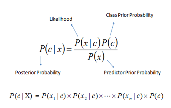
In the above image, given the training data or attributes x, the posterior probability of class c, P(c|x) follows Bayes theorem and the notations imply:
- P(c|x) is the posterior probability of class or category c given the predictor or attribute x.
- P(c) is the prior probability of a class, also known as the Class Prior Probability. It is the relative frequency of class c samples.
- P(x|c) is the likelihood i.e it is the probability of the predictor x given the class or category c.
- P(x) is the prior probability of the predictor, also called Predictor Prior Probability, and is constant for all the target classes.
After calculating the posterior probability for different assumptions, we choose the assumption or the hypothesis having the highest probability. The hypothesis with the maximum probability is known as the Maximum a Posteriori (MAP) hypothesis.
Understanding MAP Hypothesis:
To represent this mathematically, the above equation P(c|x) = (P(x|c) * P(c)) / P(x) can be written as:
MAP(c) = max(P(c|x))
or
MAP(c) = max((P(x|c) * P(c)) / P(x))
In the above equation, while computing the most probable hypothesis or the Maximum a Posteriori (MAP), we can drop the predictor prior probability P(x) as it is a constant and its purpose is only to normalize. Also, in the classification problem, we can have an even number of cases in each category or class in the training data. In this case, then the P(c) which is the prior probability of the class will be equal. Then, the P(c) can also be dropped from the equation and the final result for the Maximum a Posterior (MAP) becomes:
MAP(c) = max(P(x|c))
The estimation of P(x1, …, xk|c) = P(x1|c) * P(x2|c) *…* P(xk|c) depends on the type of variable:
- In case, the i-th attribute is categorical: The probability P(xi|c) is computed directly by taking the relative frequency of samples having value xi as an i-th attribute in class c.
- If the i-th attribute is numerical then it can be either converted to categorical and then compute the probability P(xi|c) or if we know the distribution of the variable then can compute the probability P(xi|c) using the probability density function (pdf)
- For example, if the i-th attribute is continuous then the P(xi|c) is computed through the Gaussian density function.
The assumption of independent attributes in the N****aive Bayes formula is an important step for feature engineering in naive Bayes machine learning. This implies that there is no multicollinearity present in the training dataset. We shall understand the Naive Bayes machine learning with the help of an example in the following section.
Types of Naive Bayes Algorithms
There are primarily three types of Naive Bayes algorithms: 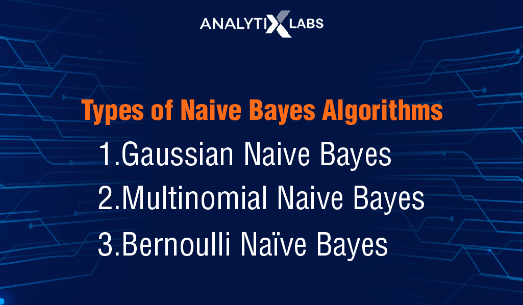
1. Gaussian Naive Bayes
It is used for continuous data where the data follows Gaussian normal distribution.
2. Multinomial Naive Bayes
It is used for data with discrete counts. It is used on data following multinomial distribution. A use-case of multinomial Naive Bayes machine learning is in natural language processing. In the text classification, this variant of Naive Bayes is applied to check how many times a word appears in the documents. The feature vector space is the relative frequency or the number of occurrences of a term.
3. Bernoulli Naive Bayes
It is applicable when the data follows multivariate Bernoulli distributions. Here, multiple features exist but the feature vector is binary, i.e. each feature has a binary value. In the case of text classification with the bag of words model,
Bernoulli Naive Bayes is implemented to check the presence of a word in a document i.e where 1 implies the word appears in the document and 0 reflects that the word does not appear in the document.
In Naive Bayes machine learning python implementation, we have the following classifiers and each of these classifiers assumes that X variables are independent of each other.
| Naive Bayes Classifiers | Distribution | Variable Type |
|---|---|---|
| Bernoulli | Binomial Distribution | Binary Categorical Variables |
| Multinomial | Multinomial Distribution | Multinomial Categorical Variables |
| Gaussian | Normal Distribution | Continuous Variables |
Representations used by Naive Bayes Models
The representation for the Naive Bayes models is probability. The two important probabilities are:
- Class labels probabilities: The probabilities of each class i.e P(c) in the training dataset.
- Likelihood or conditional probabilities: The conditional probabilities of each predictor given each class i.e P(x|c).
Let’s now look into how to prepare data for Naive Bayes.
How to prepare data for Naive Bayes
Let’s understand the algorithm by taking Naive Bayes machine learning examples. The problem statement is to check if the customer will churn or not. Below is a dummy training data of 10 customers along with the predictor variable and the corresponding target variable and a new data entry of a customer for which will find out if the customer will churn or not.
| Customer Id | Gender | Location | Marital Status | Education | Income Group | Churn |
|---|---|---|---|---|---|---|
| 1 | Male | Bangalore | Married | Post Graduation | High | Yes |
| 2 | Female | Gurgaon | Married | SSC | Low | No |
| 3 | Male | Chennai | Unmarried | Graduation | Medium | No |
| 4 | Male | Hyderabad | Unmarried | SSC | Low | No |
| 5 | Female | Bangalore | Married | Graduation | Low | Yes |
| 6 | Female | Gurgaon | Unmarried | Post Graduation | Medium | No |
| 7 | Female | Chennai | Married | Graduation | Medium | Yes |
| 8 | Male | Hyderabad | Married | Post Graduation | High | No |
| 9 | Female | Bangalore | Married | SSC | Low | Yes |
| 10 | Male | Gurgaon | Unmarried | Graduation | Medium | No |
| 11 | Male | Bangalore | Unmarried | SSC | Medium | ? |
Steps to compute the probability of an event are:
- Step 1: Calculate the prior probability P(c) for all the given classes or targets.
- Step 2: Estimate the likelihood or the conditional probability P(x|c) with each predictor variable (x) for each class ©.
- Step 3: Plug these values in the Bayes Formula P(c|x) = (P(x|c) * P(c)) / P(x) and calculate the posterior probability of class P(c|x).
- Step 4: Based on the given predictor variable, select the target class with the maximum probability.

Steps to prepare data for Naive Bayes:
1. Convert the training dataset into a frequency table like below: 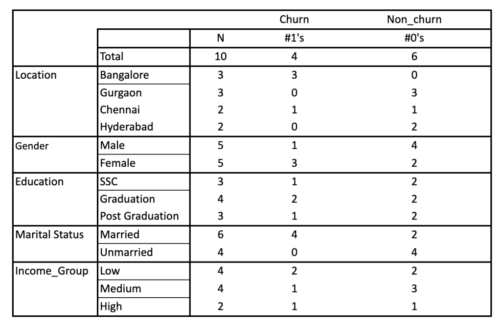 2. Create a likelihood table by finding the following probabilities:
 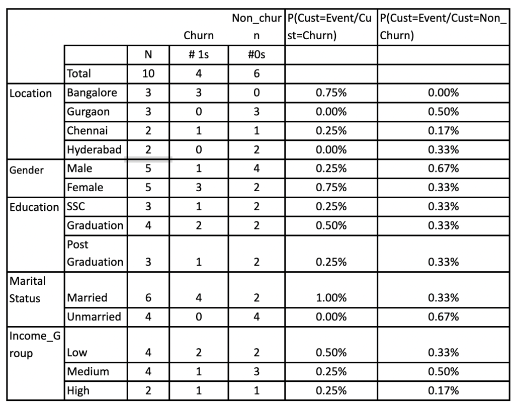 3. Calculate the posterior probability using Naive Bayesian equation for each class. One with the highest posterior probability is termed as the outcome of that prediction.
If there are missing values in the training data then those records or instances against which values are missing are not included in the frequency count for attribute value-class combinations. For classifying into labels, these attributes are not included in the calculation.
As said above the representation of Naive Bayes involves calculating class probabilities and conditional probabilities.
Class probabilities are simply the probabilities of each class i.e the frequency of records that belong to each class divided by the total number of records.
In our case of binary classification the probability of a record belonging to class 1 or to category of Churn is calculated as:
P(Class= Churn) = count(Class=Churn) / (count(class= Churn) + count(class= Not Churn))
Therefore, here the probability of class churn = 4/10 = 0.40 and the probability of class not churn = 6/10 = 0.60. Moving to the computation of conditional probabilities, which are nothing but the probability of each predictor given each class or likelihood i.e P(x|c). For instance, in the above example, the values for the gender variable are Male and Female and the target is Churn or Not Churn. The conditional probabilities for each of the gender values for each target value is calculated as:
- P(Gender = Male| Customer = Churn) = count(record with gender = Male and Customer = Churn) / count(records with Customer = Churn)
- P(Gender = Male| Customer = Not-Churn) = count(record with gender = Male and Customer = Not-Churn) / count(records with Customer = Not-Churn)
- P(Gender = Female| Customer = Churn) = count(record with gender = Female and Customer = Churn) / count(records with Customer = Churn)
- P(Gender = Female Customer = Not-Churn) = count(record with gender = Female and Customer = Not-Churn) / count(records with Customer = Not-Churn)
Using the above method, we estimate the posterior probability of both Churn and Not churn class for the given predictor gender having Male as value:
P(Churn | Male) = P(Male|Churn) * P(Churn) / P(Male)
Here, we have:
- P (Male | Churn) = 1/4 = 0.25
- P(Male) = 5/10 = 0.50
- P(Churn) = 4/10 = 0.40
P(Churn | Male) = 0.25 * 0.40 / 0.50 = 0.20 P(Not Churn | Male) = P(Male| Not Churn) * P(Not Churn) / P(Male)
- P (Male | Not Churn) = 4/6 = 0.67
- P(Male) = 5/10 = 0.50
- P(Not Churn) = 6/10 = 0.60.
P(Not Churn | Male) = 0.67 * 0.60 / 0.50 = 0.80. Based on this computation, if the attribute is male then we would expect the customer will not churn as it has a higher probability. Similarly, we can compute the posterior probability for the class based on the other conditions.
Implementation of Naive Bayes in Machine Learning: Scenarios
Some of the scenarios where Naive Bayes in machine learning is applied are:
- MultiClass Classification: With Naive Bayes’s assumption of independence between features, the technique is useful for classifying objects in multi-class. For instance, predicting if it would rain tomorrow based on temperature, and humidity. It is applicable for classifying medical data such as the detection of blood cells.
- Text Classification: A very handy use of Naive Bayes is in the domain of text data. Natural Language Processing employs Naive Bayes for text classification, detection of emails as spam or not-spam, and sentiment analysis.
- Real-time Prediction: The algorithm is efficient, having more speed is used to make predictions on a real-time basis.
- Recommender Systems: Naive Bayes classifiers help create a powerful system to predict whether a user would like a particular product (or resource).
- Credit Scoring: Naive Bayes classifiers can also be applied to predict good or bad credit requests.
We have covered the basic overview of Naive Bayes machine learning. You might still have some questions. We have covered a few in the FAQ section below. If you have any more queries, do drop them in as comments on this blog.
Learn from AnalytixLabs
You can explore our certificate course in Machine Learning and also our certificate course in data science, or you can book a demo with us.
Naive Bayes Machine Learning: FAQs
Q: How does naive Bayes work in machine learning? Based on Bayes’ theorem, Naive Bayes assumes that the predictors are independent of each other. The technique predicts the probability of different classes of the response variable. Q: What is the benefit of Naive Bayes in machine learning? Naive Bayes is relatively faster than other machine learning algorithms as it holds the assumption that the features are independent of each other. At times, speed takes precedence over high accuracy. Q: Where is Naive Bayes used? Naive Bayes is used for binary and multiclass classification. Naive Bayes machine learning for beginners is applicable for text classification, sentiment analysis, spam filtering, and recommender systems. Q: What type of machine learning is Naive Bayes? Naive Bayes is a classification algorithm and therefore is a supervised learning method. Q: What is the difference between conditional probability and Bayes theorem? Conditional probability is the likelihood or the probability of an event, given the occurrence of a previous event. Whereas Bayes’ theorem is derived via the definition of conditional probability. It is a mathematical formula used to determine the conditional probability of events. It includes two conditional probabilities offering a way to update existing predictions or probabilities based on the new or best additional evidence.