One of the most important algorithms in the field of Data Science is Logistic Regression and is among the essential algorithms learned by the students of Data Science.
Models created using logistic regression serves an essential purpose in data science as they manage the delicate balance of interpretability, stability, and accuracy in the model with great ease.
By understanding the types of business problems, statistical models’ role, the meaning of generalized linear models, etc. logistic regression can be comprehended.
The problem with understanding logistic regression is that either the explanation can be too vague, which may be fit for beginners but not good enough to have a proper understanding of the algorithm, or the explanation can be so technical and complicated that people only with a profound mathematical and statistical background can understand them which again leaves out a large chunk of aspiring data scientist who wants to have an intermediate knowledge of the topic.
This article aims to explain the logistic regression formula, its difference with linear regression, and its implementation in statistical tools such as R in a simple, easy to comprehend language.
What is Logistic Regression
Logistic Regression is better understood when it is pitted against its regression-based counterpart- Linear Regression. But before that, it is important to understand where Logistic Regression individually lies in the world of Data Science algorithms.
To understand this, let us first understand the world of algorithms. All the algorithms at their heart hold a formula and are used to create models.
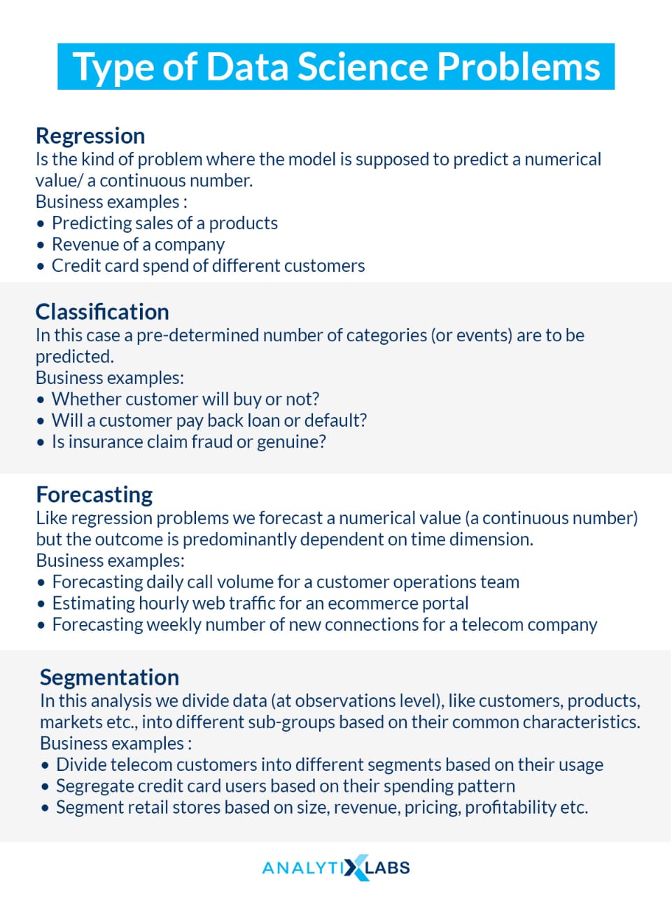
Foremost, these methods can be understood based on different data science problems they solve, and this broadly can be categorized into regression, classification, segmentation, and forecasting problems. We can understand these in simple terms as following:
Regression: Regression is the kind of problem where the model predicts a numerical value/ a continuous number. Business examples:
- Predicting sales of a product
- Revenue of a company
- Credit card spends of different customers.
Classification: In this case, a pre-determined number of categories (or events) will be predicted. Business examples:
- Whether customers will buy or not?
- Will a customer payback loan or default?
- Is insurance claim fraud or genuine?
Forecasting: Like regression problems, we forecast a numerical value (a continuous number), but the outcome is predominantly dependent on the time dimension. Business examples:
- Forecasting daily call volume for a customer operations team
- Estimating hourly web traffic for an eCommerce portal
- Forecasting weekly number of new connections for a telecom company
Segmentation: In this analysis, we divide data (at observations level), like customers, products, markets, etc., into different subgroups based on their common characteristics. Business examples:
- Divide telecom customers into different segments based on their usage
- Segregate credit card users based on their spending pattern
- Segment retail stores based on size, revenue, pricing, profitability, etc.

The second way through which models can be categorized is algorithms. Different kinds of algorithms give birth to different models, and these models can broadly be divided into 3 major categories – Statistical Models, Machine Learning Models, and Deep Learning Models.
While Machine Learning and Deep Learning models use purely mathematics-based algorithms, statistical models use formulas that use the concepts of statistics for their functioning.
To solve the aforementioned 4 types of data science problems, we can virtually deploy any of these 3 models.
Lastly, the models can be divided based on the type of business problem they solve, and among these are Strategic problems and Operational problems.
Strategic problems are those problems where models are expected to provide details as to how they are coming at a particular prediction (i.e., high level of model interpretability), operation problems, on the other hand, require those models that are reliable, fast, and are highly accurate even if they may not provide a high level of interpretability.
With this understanding, it is easy to understand what is logistic regression. Logistic Regression is an algorithm that creates statistical models to solve traditionally binary classification problems (predict 2 different classes), providing good accuracy with a high level of interpretability.
While machine and deep learning-based algorithms are often used to solve operational problems, models created using logistic regression are used to solve strategic problems as they provide coefficients in their output through which a great deal of information can be figured out.
However, to properly understand the logistic regression formula, the best way is to compare it with Linear Regression and understand their differences with examples.

Comparison with Linear Regression, Formula & Equations
Linear Regression is the most common algorithm for solving regression problems, i.e., where continuous numbers are predicted. Now, suppose we introduce a classification problem or, to be more precise, a binary classification problem (i.e., where two categories are to be predicted – 0 and 1). In that case, the immediate question that runs into people’s mind is, what if we use linear regression to solve such a problem as encoded categories are numbers only. Linear regression can very well predict numbers.
Related: What is Linear Regression In ML? With Example Codes
In order to understand this and consequently the need for introducing logistic regression, we have to pay attention to the major assumptions of linear regressions, which are the following:
- The dependent (Y) variable should be normally distributed.
- X should be correlated with Y
- Minimal correlation between the independent variables (multicollinearity check using PCA or Factor Analysis)
- Data should have no missing values.
- There should be no outliers in the data.
Now, to apply linear regression to data where the Y variable has two categories (that we need to predict), we need to make sure that all the above-mentioned assumptions are fulfilled. We now check all such assumptions one by one.
The Y variable in the case of a binary classification problem cannot be normally distributed. It is not made up of continuous numbers in the first place, making it almost impossible to have any distribution other than Bernoulli distribution.
The second assumption can be partially fulfilled. We can traditionally find a correlation between two continuous numbers, while finding a correlation between numeric and categorical variables can be difficult but not impossible.
The third, fourth, and fifth assumptions are related to the X variables and can be fulfilled easily. Thus, it is majorly due to assumption #1, i.e., the Y variable not being normal, causing the linear regression not to fit such data.
This is where the concept of the Generalized Linear Model (GLM) kicks in, which allows for the Y variable to transform using a link function through which we can establish a relationship between the X and the Y variable and can come up with some form of a prediction.
These link functions can be of many types, with the most common being logit and probit. When the logit link function is used to fit a linear equation on the data where the Y is not normally distributed, then such a linear model is known as a Logistic Regression model.
Before proceeding with the Logistic Regression formula, the reader must be familiar with one statistical concept. Only then the working of logistic regression can be understood, which is odds. It can be understood from a simple example:
For example, if there are two cricket teams: India and Australia, and if we say that the odds of India winning is 3:1, then in the simplest understanding, this means that if both these teams play 4 matches, then 3 will be won by India while Australia will win one.
Therefore, Odds is nothing but the probability of an event happening divided by the probability of that event not happening. Thus, India’s odds are P(India Winning) / P(India Not Winning).
So if we know that India’s probability of winning a match is 75%, then the odds of India winning will be- 75/25 = 3, i.e., the odds are 3:1. Thus, if we know the probabilities, we can know to find the odds.
Thus, logistic regression comes up with probabilities for the binary classes (categories) using a concept known as Maximum Likelihood Estimation.
Through these probabilities, we can come up with the odds. Now, why coming up with odds is so important can be understood by understanding the Logistic Regression equation.
According to the generalized linear model, a logit function can make the Y variable normal, thus fulfilling the assumption for fitting a linear model.
The logit function states that the log of odds can be considered a normally distributed Y variable. Now, this brings us to the logistic regression equation, which is :
exp(mx+c) / 1 + exp(mx+c) which allows us to fit a sigmoid curve. Just like generalized linear equation mx+c allows us to fit a straight line to come with probabilities for the Y variable classes, a sigmoid curve fits the best as it expresses the relationship between a numerical X and a binary Y perfectly.
Now, to prove how logit function works and how the assumption of normality is fulfilled, we can understand the equation in the following way:
- Sigmoid curve = probabilities (p) = exp (mx+c) / 1+exp(mx+c)
Now to prove that a linear model can be fit, we write the equation in the following way:
- p / 1-p = exp(mx+c)
- log(p/1-p) = mx+c
- if, z = log(p/1-p)
- then, z = mx+c
Therefore, we can build a simple linear model and using it. We can calculate the value of p by running some optimization algorithms. Here, the z is known as the log of odds.
Therefore,
- log(odds) = mx+c
- p = log(p(y=1) / p(y=0)) = mx+c
Thus, Y is transformed into log(p(y=1) / p(y=0)) i.e. a log of odds and as stated earlier, as per generalized linear model, a log od odds can be considered as a normal. Thus a linear equation is made to fit on this transformed Y variable (transformed using the logit function).
As mentioned earlier, logistic regression doesn’t predict classes of the Y variable but rather predicts the probability of the classes, making the method of evaluating a logistic regression model much different from a linear regression model.
Unlike Linear Regressoon’s accuracy metrics that provide a single, stand-alone value to define the model’s accuracy, for logistic and any classification model for that matter, we need to take multiple things into account.
Apart from metrics such as Area Under the Curve value and KS statistic, most of the accuracy metric depends upon how the classes are defined.
Once the probabilities are made available by logistic regression, we need to develop a threshold value that allows us to define the predicted class. For example, if we set the threshold value at 0.8, then the observation with the predicted probability greater than 0.8 will be assigned with class 1; otherwise, 0.
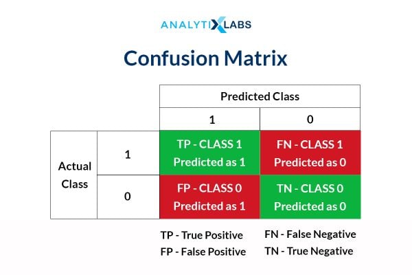
This gives birth to the confusion matrix concept, and if we manipulate the threshold value such that most of the predicted classes are of the majority class, then a simple accuracy where it is counted how many times a class is correctly predicted increases dramatically.
However, this is the wrong way of calculating accuracy as we need to look at the wrongly predicted classes. Therefore, a confusion matrix provides us with a better picture.
This allows for a range of accuracy metrics to be calculated, such as sensitivity, specificity, precision, etc. However, their values also depend on how the threshold is set, and this, in turn, brings the concept of various ways through which the right cut-off (threshold) value can be determined, such as ROC Curve and Decile Analysis (KS Table). Thus, the method of evaluating a logistic regression model is significantly different from a linear regression model.
There are certain things in terms of the advantages and disadvantages that both linear and logistic regression share with each other. Logistic Regression, just like Linear Regress, is a statistical algorithm that allows for the creation of highly interpretative models.
They are easy to implement and are relatively stable. However, they both suffer from a lack of accuracy, especially if the data is in high dimensions and requires several fulfilled assumptions.
Examples of Logistic Regression in R
Logistic Regression can easily be implemented using statistical languages such as R, which have many libraries to implement and evaluate the model. Following codes can allow a user to implement logistic regression in R easily:
- We first set the working directory to ease the importing and exporting of datasets.
>> setwd("E:/Folder123")
- We then import some datasets.
>> df
<- read.csv('dataset.csv')
- To comply with the assumption, it is better to check if there are any outliers or missing values, and if there are, then this must be treated.
Missing values can be treated by using median value imputation.
>>
miss_treat = function(x){
x[is.na(x)] = mean(x,na.rm=T)
return(x)
}
>> df =
data.frame(apply(df, 2, FUN=miss_treat))
Outliers can be removed by restricting the higher values at 99th and lower values at the 1st percentile.
>> outlier_treat <- function(x){
               UC
= quantile(x, p=0.99,na.rm=T)
               LC
= quantile(x, p=0.01,na.rm=T)
               x=ifelse(x>UC,
UC, x)
               x=ifelse(x<LC,
LC, x)
return(x)
}
>> df =
data.frame(apply(df, 2, FUN=outlier_treat))
- To make the model stable and reduce the chances of overfitting, the data is split into train and test dataset where the logistic regression model is developed on the training dataset. In contrast, it is evaluated on the testing dataset.
>> train_ind
<- sample(1:nrow(df), size = floor(0.70 * nrow(df)))
>>
training<-df[train_ind,]
>>
testing<-df[-train_ind,]
- Under the stats library, the glm function is provided to create a logistic regression model. Here the Y variable is provided before the ~ symbol. The names of the independent variables are provided after it and the type of link function we want to choose, which will be logit for implementing logistic regression.
>>
logreg <- glm(Y~var1+var2+ var3+var4+var5,data = training, family =
binomial(logit))
- The summary functions allow for finding the coefficients and evaluating the importance of the independent features.
>> summary(logreg)
- The coefficients can also be individually assessed by using the coefficient function.
>> coeff<-
logreg $coef
- To finally come up with the predicted probabilities, the predict function is used. We can also append the prediction results with the original dataset too.
>>
train<- cbind(training, Prob=predict(fit2, type="response"))
- Logistic Regression can be evaluated in multiple ways. Many libraries provide various functions for evaluating such classification models.
>> library
(InformationValue)
>> library
(Metrics)
>> library(pROC)
>> library
(e1071)
The following are the common methods to evaluate a logistic regression model-
- Concordance
>> Concordance(train$Y,
train$Prob)
2. AUC Score
>>
roc_obj <- roc(train$default, train$Prob)
>>
auc(roc_obj)
3. Confusion Matrix
>>
pred_mod_log <- ifelse(train$Prob > 0.5,1,0)
>>
train_Y <-training$Y
>>
confusionMatrix(pred_mod_log, train_Y)
(Calculating class-dependent accuracy metrics)
4. Accuracy
>> Accuracy
<- accuracy(train_Y,pred_mod_log)
5. Sensitivity
>> Senstivity
= InformationValue::sensitivity(train_Y,pred_mod_log)
6. F1 Score
>> f1
<- Metrics::f1(train_Y,pred_mod_log)
7. Specificity
>> specificity
= InformationValue::specificity(train_Y,pred_mod_log)
- Once the model’s accuracy is determined, we can also tweak the cut-off to come up with new classes. Optimal threshold values can be found using the ROC Curve or KS table.
ROC Curve (Method 1)
>>
cut1<-optimalCutoff(train$default, train$Prob, optimiseFor =
"Both", returnDiagnostics = TRUE)
>> cut1$optimalCutoff
ROC Curve (Method 2)
>>
roc_obj <- roc(train$default, train$Prob)
>> coords(roc_obj,
"best", "threshold", transpose = TRUE)
KS Table
>> ks_table<-ks_stat(train1$default,
train1$Prob, returnKSTable=TRUE)
All the above-mentioned codes can help develop a logistic regression-based predictive model, identify the best cut off value, and evaluate the model for different cut-off values.
Logistic Regression is among the most widely used and accepted algorithms for solving a binary classification problem.
One must know that logistic regression can solve the multiclass problems, too; however, theoretically, it works as a binary classifier only.
While the implementation of logistic regression is straightforward, it takes experience and a good understanding of this algorithm’s inner working to master it and gain highly accurate results from it.
However, once this statistical algorithm is mastered, logistic regression’s level of information is unparalleled. It is the reason that even after the introduction of the machine vs deep learning algorithms, the popularity of logistic regression has not diminished.
The fulfillment of multiple assumptions to run it soundly can pose a bit of a challenge. However, once the data is cleaned and prepared, logistic regression can provide extremely stable results, especially if multicollinearity and outlier problems are addressed. Running Logistic Regression in R is particularly easy. No matter what kind of a project it is, it is always advisable to implement a logistic regression model if there is a classification problem.
You may also like to read: How to Choose The Best Algorithm for Your Applied AI & ML Solution.


![Understanding Binary Tree: Guide to Binary Tree Implementation in Python[with codes] binary tree in data structure](https://www.analytixlabs.co.in/blog/wp-content/uploads/2024/10/Binary-Tree-in-Data-Structure-01-370x245.jpg)


