Fundamentals of Statistics for Data Science

Introduction to Statistics

Statistics is among the most widely used and important disciplines of study proven to be indispensable in numerous domains such as Engineering, Psychology, Operational Research, Chemometrics, etc. Among the most dependent statistical disciplines is Data Science, which is why for having an in-depth understanding of it, Statistics should be understood in great detail.

The term statistics is often misunderstood, and this is the reason that first, we need to get an evident understanding of it. To understand basic statistics for data science, we first must understand and get familiarized with a few basic terminologies.

Population

Understanding the basic statistics for Data Science begins with the most common concept, “Population”. A population can be understood as the total number of individual humans, other organisms, or any other object that makes up a whole. With this understanding, the underlying conditions are critical in determining the number of objects/items, etc., that will form the population. If we talk about the Apple Laptops manufactured in September 2013 in a particular factory in China, then the number may not be as large as the total number of computers presently active in the world. Thus, the population may or may not be large as this depends on the conditions which define what is to be considered as the population.

Parameter

Numerous mathematical calculations can be performed on the population, such as finding the most common item or value occurring in the population or finding the average. All such arithmetic operations that allow us to define the population in simple numeric digits are provided with the term parameter. For example, if we want to know the average age of all the people living in a village. If there are 200 people in that village whose age we can capture successfully, then this average age will be called a parameter. It will be called so as its value has been calculated using the complete population information.

Sample

In simplest terms, a sample is nothing but a subset of the population (that ideally represents the population). The samples can be of various types, such as

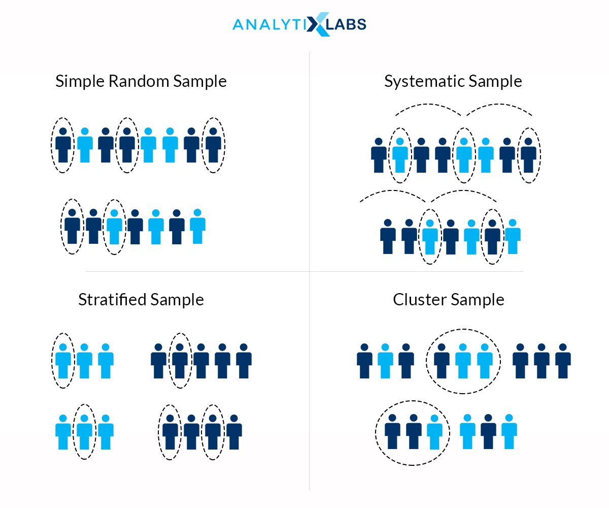
1. Random Sample: Samples generated by randomly picking objects from the population and random means without any bias or preconceived conditions. Here every object (or whatever the subject is in the population) gets an equal opportunity to be selected as a part of the sample.
2. Stratified Sample: Here, the samples are created by considering the underlying groups that could be found in the population. For example, if we are collecting a sample of cars on roads and 40% hatchback and 60% sedans, then we will follow the same stratification while creating the sample.
3. Convenience Sampling: Among the most widely used method of creating a sample, under this methodology, samples are not created by chasing after the subjects. A typical example of this would be online surveys or samples created through feedback forms, etc. The subjects will provide information.
4. Clustered Sample: This form of sample creation is most commonly conducted in collecting data for Exit polls, TRP calculation, advertisement placement, etc. Here the geographical area is divided where from each geographical entity, a stratified or random sample is created.

One must keep in mind that no method is intrinsically better or worse than the other, and are just different ways of creating a sample that suits different requirements.

The next logical question could be to question the need to create a sample in the first place. Why do we need to create a sample when we have the population, and this has few obvious answers.

• Firstly, there can be a situation where capturing the population information is nearly impossible. For example, to know the age of each human being on earth. Finding the average of 7 billion numbers may not be an impossible technological task but to obtain such information is extremely tough. Here the population is highly dispersed, which makes it difficult for us to obtain the complete data.
• The other reason can be when we have population information, i.e., a bank having many branches throughout the world. Each has hundreds of accounts, which in turn makes numerous transactions. While such data may be available in the bank’s server, doing any operation on such population data can be challenging because of its sheer velocity and volume.

And with the above understanding, we can now finally understand the term statistics.

Statistics are the numerous arithmetic operations performed on the sample that allow us to summarize and make inferences about the population. While this is one of the understandings, which is sample-oriented, statistics can also be understood as simply a form of study that allows us to take data and define or summarize it using numerous techniques. 

There is a requirement to know basic statistics concepts for data science as the discipline requires us to define data, and here are statistics in the best tool.

Scope of Statistics in Data Science

To know the statistics for data science, one first needs to understand the role statistics plays in this field. A Data Science project has numerous stages. Statistics play a minor in each stage’s major roles, so knowing the basic statistics concepts is considered mandatory. Following are among the few common roles that statistics play in the field of Data Science-

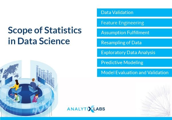
Data Validation

As we often work on samples, it is important to know if the sample represents the population or not, and this is where statistics play an important role. Numerous statistical tests can help identify if the sample is good enough to make decisions based on the insights it is providing us.

Feature Engineering

Undoubtedly one of the most important phases of any Data Science project is performing feature engineering. Feature Engineering can be understood as preparing numerous variables, aka features, to make them worthy of being used in any model. This feature engineering depends heavily on statistics.

a. Outlier Treatment

To identify outliers and find the appropriate upper and lower bound values, statistical concepts such as percentiles and Inter Quartile Ranges are to be understood. They help us understand where the bulk of data lies and what data points can be considered an anomaly or extreme value in nature that can act as noise during the implementation of an algorithm.

b. Missing Value Treatment

Numerous statistical concepts are needed when dealing with missing values in the data. Traditionally, when the data was often survey-based, missing values used to be a highly commonly occurring problem, which was solved using statistical concepts. While today, sophisticated Machine Learning methods do exists to deal with missing values, the traditional, easy to implement, and reliable way of dealing with missing value is continued, which is done by performing imputation. Imputation is the replacement of missing values by some statistically calculated value that does minimum damages to the data’s overall structure.

c. Feature Reduction

The curse of Dimensionality is a highly common phenomenon in Data Science. With the increase in the number of features/variables/columns, the model tends to become more unstable and can become a victim of overfitting. In part, this problem is also due to multicollinearity, which can again commonly occur, especially if the data is in high dimensions. This is where feature reduction methodologies come in, among which a large number belongs to the field of statistics. These include the use of various filter methods that include:

• Establishing a correlation between dependent and independent variables
• Analysis of the correlation matrix between the independent variables to check for multicollinearity
• Performing Statistical tests between dependent and independent variables and between two independent variables

Several wrapper methods also use statistical concepts to perform feature reduction, such as

• Variance Inflation Factor to check for multicollinearity in the data
• Recursive Feature Elimination to find the least important variables by assessing their impact on the dependent variable
• F Regression / Univariate Regression to find important features in an isolated space
• Stepwise Regression (both direction) to look for important and unimportant features simultaneously

Assumption Fulfilment

To fulfill the requirements of algorithms, statistics come in handy. For example, algorithms such as Linear Regression require the dependent variable to be normally distributed. Simultaneously, it also requires the independent variables to have a strong correlation with the dependent variables. All these assumptions can be assessed and, at times, fulfilled by the use of statistics.

Resampling of Data

Especially during classification problems, the class imbalance can create deep problems. A class imbalance is when certain categories of the dependent variable are over or under-represented. This is where statistics play an important role as it allows for this problem to solve by using the resampling of data that includes oversampling, undersampling, hybrid sampling, etc.

Exploratory Data Analysis

To perform a basic statistical analysis of data and visualize the data, statistics play a major role. When a large amount of data is to be analyzed, there is a requirement to develop simple, single-digit numbers that can provide a great deal of information about the data. This is where the data is aggregated, summarized, etc. Using descriptive statistics, and relationships between variables are established, providing key insights about the data.

Predictive Modeling

Perhaps the most common and important application of statistics in Data Science is the role it plays in creating predictive models. While there are Machine Learning and Deep Learning models, no one can take the place of statistical models when it comes to reliability, the minimum level of accuracy, and, most importantly- interpretability. Predictive models such as Linear Regression and Logistic Regression predict numbers and categories and provide a great deal of transparency while doing so, making them a favorite for domains such as Marketing, Finance, or whenever strategic problems are to be solved.

Model Evaluation and Validation

A less discussed role of Statistics in Data Science is how it acts as a checkpoint for models giving us information regarding how the model works. Numerous model evaluation metrics use statistical concepts such as

• R-squared (R²)
• Adjusted R Squared (Adj R²)
• Mean Absolute Percentage Error (MAPE)
• Root Mean Squared Error  (RMSE)
• KS statistic (Kolmogorov-Smirnov Statistic)
• Decile Analysis
• Analysis of Residuals
• Precision
• Recall aka Sensitivity
• Specificity
• ROC Curve
• Gini Coefficient
• F1 Score
• Concordance

Thus, statistics play a role in almost every stage of Data Science. While the level of involvement and complexity varies, there is hardly any stage where statistics are completely absent.

Categories in Statistics

After understanding the basic statistics concepts, we will now see the numerous ways through which Statistics can be categorized. These categorizations can help in getting a better insight into the statistics for data science. Among the two most common categories are the Descriptive v/s Inferential Statistics and  Frequency v/s  Bayesian Statistics.

Descriptive vs. Inferential

The most common way of dividing especially the traditional statistics, is between Descriptive and Inferential.

• Descriptive Statistics

This form of statistics deals with the population as well as the sample. As the name suggests, descriptive statistics are used to describe the features and characteristics of the data. Here, the facts regarding the data are exposed, giving us a quick glimpse of the data. Descriptive statistics are most commonly used in Exploratory Data Analysis and various forms of reporting. Various statistics measures (to be discussed ahead) are used to describe the data, and all such measures form the descriptive statistics.

• Inferential Statistics

Under Inferential Statistics, we go one step ahead. Rather than merely describing the data or stating the facts about it, we draw some conclusions about the population based on the sample at hand. Under Inferential Statistics, we mainly work with samples, draw “inferences” about the population, the relationship between samples, and find the statistical significance of data and changes in the data.

Frequential vs. Bayesian

The next way through which statistics can be categorized is between Frequential and Bayesian.

• Frequential Statistics

This is the form of statistics where we use probability distribution to come up with any statistical answer. Here the concept of Hypothesis testing is used. The conclusion is based on the probability of how common or rare a value can be found in a particular distribution, thus, finding the probability of an event happening. The concept of prior is not involved in such kind of statistics. This is generally the traditional form of statistics with which most people are familiar.

• Bayesian Statistics

It is a more peculiar form of Statistics that doesn’t only work on the concept of the probability distribution. Bayesian Statistics includes the concept of prior, which can be understood as a concept where some information before considering the actual events is considered. A typical example is of dice rolled a hundred times, and based on the outcome, we find the probability of getting 1 in the outcome. However, if the dice are loaded to the land on 1, i.e., it is manipulated in such a way that the chances of getting 1 in the outcome are higher then this information known before the evidence (the actual outcomes) can be considered under Bayesian Statistics allowing us to have to a more informed and confident answer.

Basic Statistics Concepts

Some statistical concepts are essential for understanding the common statistics topics for data science. The following are the most relevant concepts-

Probability Distributions

In statistics, we can assess how it is spread or dispersed or distributed when we collect data. This collection of values or distribution can be represented or visualized using graphs such as histograms. Statisticians, over time, have come up with the common distributions. They have developed associated probability distribution that allows us to know the probability of finding a value in a particular distribution type. Common types of probability distribution include-

• Gaussian (Normal)
• Student’s t
• Log-Normal
• Poisson
• Binomial
• Bernoulli
• Uniform
• Chi-Squared
• Exponential

For example, Gaussian, aka Normal Distribution, has the associated Standardized Normal Distribution, a probability distribution. Corresponding to it, we have a Standardized Normal Probability Distribution table that allows us to know the probability of finding value in our data (if our data is normally distributed).

Central Limit Theorem

As per traditional and theoretical statistics, if we take a large number of samples from the population (theoretically 30+ samples), then the distribution of this sample is (almost) normally distributed even if the population’s distribution was not normal (Refer Bean Machine). Along with this, it states that the mean of this sample distribution will coincide with the mean of the population distribution.

Related: Application of Central Limit Theorem – An Illustration

Three Sigma Rule

The 3 sigma rules state that if the data distribution is normal (Gaussian), then we can know how much data will be within certain bands around the mean or, in other words, we can know the area under the curve by using the standard deviation. As per the 3 sigma rule, if we move one standard deviation above or below the mean, we capture 34.1% of data making the total data between one standard deviation above and below the mean at roughly 68.27%. Similarly, if we move two standard deviations above the mean, we get an increase of 13.5% of data making the total amount of data between two standard deviations above and below the mean at 95.45%. Finally, if we further move one more standard deviation, then we capture an additional 2.35% of data making the total to be 99.73% data between three standard deviations above and below the mean.

Univariate, Bivariate, and Multivariate Statistics

Statistics can be performed using a single variable, two variables, and even multiple variables. When we use a single variable to perform statistics, where most of the descriptive statistics lie, such statistics are univariate statistics. When we use two variables, which is generally the case with inferential statistics where we are trying to assess the relationship between the two samples, this statistic is commonly called a Bivariate Statistics. Finally, when we have multiple variables where we simultaneously assess the relationship using multiple variables, this is known as multivariate statistics. For example, linear regression is a form of statistics where we try to assess the relationship of multiple independent features with a single dependent feature.

Hypothesis Testing

The statistics for data science use numerous inferential statistics concepts where there are numerous statistical tests, i.e., ways of analysis. These tests are performed under two main hypotheses. One of the hypotheses known as the Null hypothesis is that there is no statistical difference or change. Common Null Hypothesis include-

• No Statistical difference between the population mean (or hypothesized value) and the sample mean
• No Statistical difference between the means of two samples
• Two variables do not have any statistical relationship and do not influence each other.

The other hypothesis is known as the Alternative Hypothesis, which stands for change. The common alternative hypothesis include

• There is a statistical difference between the population mean (or hypothesized value), and the sample mean
• There is a statistical difference between the means of two samples.
• Two variables have some statistical relationship and influence each other.

The statistical tests’ idea is to reject or accept the null hypothesis, thereby giving us some insights regarding the data.

One-tailed and Two-tailed tests

The hypothesis tests can be one or two-tailed depending upon the type of alternative hypothesis. If the alternative hypothesis states that the population means/hypothesized value/mean of a sample is greater than (or less than) the other sample’s mean, then such a test is known as the One-tailed test. On the other hand, if the alternative hypothesis states that the difference can be in either direction (less than as well as greater than), then such a test is called a Two-tailed hypothesis test.

Standardization

The process of converting values to a metric free value is known as standardization. One of the most common ways of standardization is finding the z scores of values where z scores are the values in terms of standard deviation units. These z-values can be used to find how much area is under the curve in a standardized normal probability distribution table.

p-value and alpha value

p-value stands for probability value. Under probability distribution, once a value is identified on the probability distribution, then the area left on either side is known as the probability. If the value is close to the mean, it would have a large amount of area under the curve, i.e., a high p-value, which indicates that it is a common value. The probability of finding such valuable data is also high. On the contrary, if the value is far away from the mean, then the p-value will be low, indicating the probability of finding such a value in the data is low. This concept is used in hypothesis testing to accept or reject the null hypothesis. To define if the p-value is high or not, we decide an alpha value. If the p-value is higher than the alpha value, then we consider the p-value to be high, indicating that the value is commonly found in the data. Hence, it is not statistically significantly different from the mean allowing us to accept the Null Hypothesis.

Different Measures in Statistics

To describe a cube, we have to measure the length, breadth, and height of it. Similarly, if we have to describe the data statistically, we have to measure the data, and there are four such common measures in statistics.

Measure of Frequency

Here we count how many times a value appears in the data. This is the most common and simplest measure. Here we create Frequency tables, pie charts, and bar charts from visualizing it. However, for numerical data, the most effective way to visualize it is through histograms.

The Measure of Central Tendency

The typical way in which we summarize the data is by finding its central point. This central point is calculated in numerous ways, such as Mean, Median, and Mode, which form the measure of the data’s central tendency.

Mean

It is the simple arithmetic average of the data

Median

It is that value that marks the 50^th percentile, i.e., the central value or middle value when we arrange the data in an ascending/descending order

Mode

It the most commonly occurring value or the value with the highest frequency

Measure of Dispersion

For example, we have a record of two cricket batsmen

Batsman-A	Batsman-B
50	0
40	150
60	10
70	130
30	7
40	10
50	120
29	20
80	0

If we calculate the mean of their score, then it comes out to be roughly the same (50); however, which batsman is more consistent can be found by analyzing the dispersion of the values, and this is where the measure of dispersion helps. The most common measures of dispersion include-

Range
Finding the difference between the maximum and minimum value. This can be problematic as outliers can affect it adversely.

Interquartile Range
Finding the difference between percentile 75^th and 25^th or Q3 and Q1. Here as we don’t use all the values, this method cannot be considered a reliable method for calculating the dispersion.

Variance
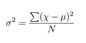
Variance is calculated by finding the difference between the value and the mean aka deviation and then taking its square (as without squaring, the sum of deviation is always 0). We then sum all these squared deviations and divide it by the count of values.

Standard Deviation
The problem with variance is that it changes the unit of the value. If the values are in km, then the variance will be in km^{2, which} is not very feasible. To correct this change, we take the square root of it, which makes the result be called Standard Deviation.

Measure of Shape
As mentioned earlier, the distribution of data can be found by plotting a histogram. This helps in revealing the shape of the distribution of the data. By analyzing the shape, we can quickly gain good insights regarding the data and its distribution. The shape can be divided into two parts- Symmetrical and Asymmetrical.

Symmetrical
If we divide the data from the middle of the distribution, then the remaining left side is the right side’s mirror image. The most common symmetrical distribution is Gaussian distribution, where the mean is the same as the median, which is the same as the mode. This allows for a symmetrical bell-shaped curve.

Asymmetrical
When the distribution is skewed, i.e., the distribution is tilted on either side, the distribution is known as Asymmetrical. Such asymmetrical distribution can be found when the data is skewed. If the data is left-skewed (negative skewed) mode is greater than the mean and right-skewed (positive skewed), the opposite is true.

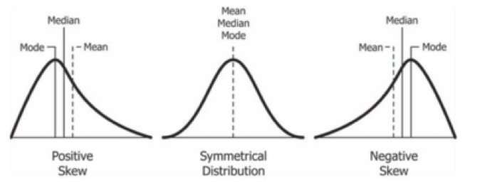
All such measures describe some or the other aspect of the data and are commonly used under the descriptive statistics to define the data’s features. While some focus on the central or most commonly occurring value, others focus on how the data is spersed, distributed, and their shape providing us a holistic view of the data.

Different Analysis in Statistics

Numerous analyses can be performed with the use of statistics. Most of them can be performed by using traditional bivariate inferential statistical. In contrast, others are a bit more complicated and can factor in multiple variables or prior calculations. These methods form the common statistics topics for data science and allow for easy statistical analysis of data. Following are the most common analysis-

One Sample t-test

These statistical tests allow us to analyze if a sample is statistically the same as some hypothesized value or some population mean or not. We can also use Z-test here, however, as the results from both these tests are almost identical if the sample size is large enough (One-Sample t-tests works fine even if the sample size is less than 30 and works same as a Z test if it is more than 30) we mostly use this test.

Dependent t-test aka paired t-test

Such a test allows us to analyze if two samples (mainly belonging to them before an event and after an event situation) are statistically the same or not. Here we compare the mean of both the samples by running hypothesis tests. If the Null Hypothesis is accepted, then the samples are said to be the same, and no change is observed.

Independent t-test

Here a sample is divided into two parts based on some categorical variables, i.e., the data is divided into two independent groups to test if they are statistically the same or not. Unlike the dependent t-test where the sample size is the same, this test’s sample size can vary.

One Way Analysis of Variance

Similar to the Independent t-test, when the data is divided into more than two independent groups, then this test is used. Here we analyze the variance between as well as within the groups. If the variance within the group is low and between the groups is high, then the groups are said to be statistically significantly different from each other.

Chi-Squared test

To analyze if two categorical variables are related to each other or not, i.e., they influence each other, and such a hypothesis test is performed. Here a chi-square value is calculated, which is the sum of the difference between the observed frequencies and the expected frequencies. If this difference is large, then we consider the variables to be influencing each other.

Correlation

It helps us in analyzing the relationship between two numerical samples/datasets. The relationship can be positive or negative, or none. If one variable increases and the other does the same perpetually, then this indicate a positive relationship. A negative relationship is when, as one sample increases in its value, the other decreases. There can be no relationship between the two samples, where the values in one variable increases or decreases randomly with no connection with the other sample.

Multivariate Linear Regression

This form of analysis allows us to come up with predictions regarding a numerical variable based on certain predictors. While the variable to be predicted is known as the dependent variable (or the Y variable), the predictors are known as the independent variables (or the X variables). Here for each predictor, we come up with coefficients that allow us to establish how they influence the Y variable. The relationship between the X and Y variable is summarized using the equation Y = bx+c where Y is the dependent variable, b is the beta or coefficient, x is the independent variable or the predictor, and c is the constant.

Bayesian Theorem

Numerous methods use the Bayesian theorem to come up with predictions. One of the algorithms is Naïve Bayes that uses Bayesian statistics to come up with the solution. Here the prior is also considered in the formula to predict the probability of an outcome. The formula for performing such an analysis is

Basic Statistics for Data Science can be understood easily by focusing on certain key statistical concepts. While the list of such concepts can go very long, the key concepts mentioned in the article can provide the initial understanding before one decides to deep-dive into the stream of statistics. Knowing statistics is highly important as it affects every aspect of Data Science. Knowing the key statistics for data science can help boost one’s career and gain a deeper understanding of the field. While descriptive statistics is important for performing exploratory data analysis, reporting, and visualization, Inferential Statistics, Regression, and Bayesian Statistics help in the advanced analysis of data by understanding the relationship between the data and even quantifying this relationship to come up with predictions making statistics an inseparable part of Data Science.

You may also like to read:

1. Top Data Science Courses & Free Resources

2. Data Science vs. Computer Science; Skills & Career Opportunities